Turn a Grid of Numbers into a Picture in Excel
Data bars and colour scales from the keyboard, live updates, and the total-row mistake that ruins data bars.
- The problem
- Totals
- Data bars
- Colour scales
- Live updates
- The total-row trap
Step by step
1. The problem
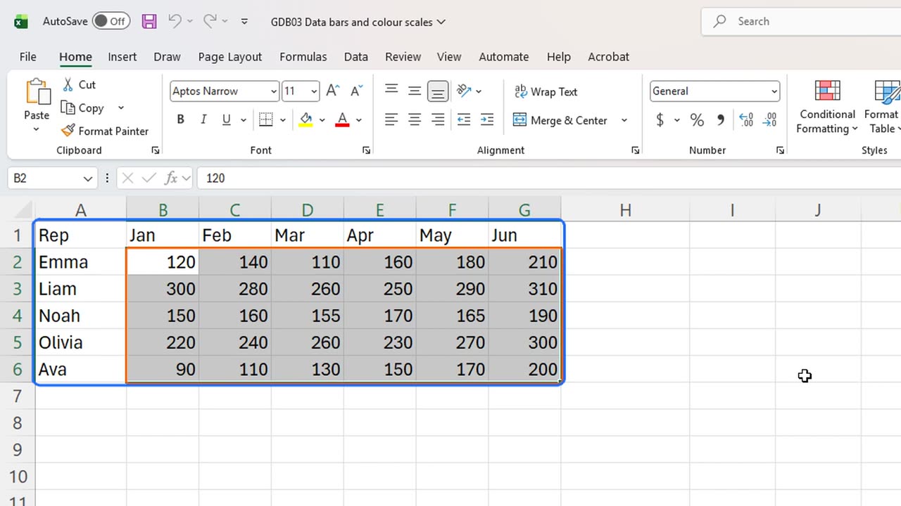
Thirty numbers, and you cannot tell who is winning. Two features turn this grid into a picture in about ten seconds.
2. Totals
First, a total for each rep. In H1, type Total. In H2, type equals SUM of B2 to G2.
Drag the fill handle down to row six, and every rep has a total.
=SUM(B2:G2)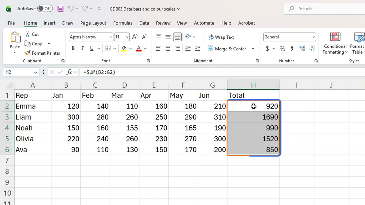
3. Data bars
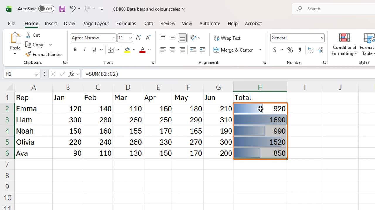
Now the first secret: data bars. Select the totals, then press Alt, H, L, and D. That opens Conditional Formatting, Data Bars.
Press Enter to take the first style.
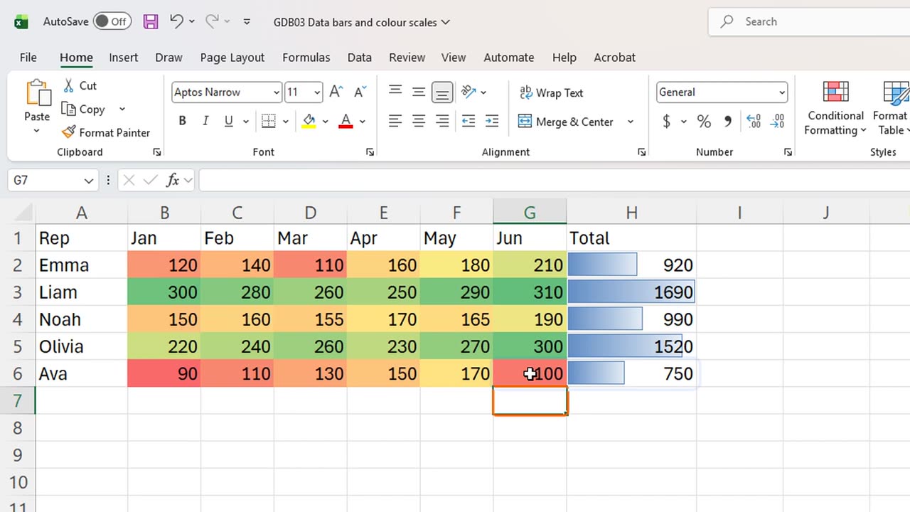
Every total now carries a bar, scaled to the largest value. Liam is clearly ahead, and Ava clearly behind, without reading a single number.
4. Colour scales
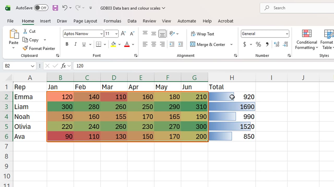
The second secret is a colour scale, which works like a heat map. Select all the monthly numbers, and press Alt, H, L, and S.
Enter takes the first scale: green for high, yellow in the middle, red for low.
Now patterns jump out. Liam is strong every month. Ava starts in the red, but look how her row climbs from red toward yellow month after month. A number grid never tells you that story so fast.
5. Live updates
Both formats are live. Change a number, and the colours and bars follow. Type one hundred in Ava's June.
June turns red, and her bar shrinks at once.
6. The total-row trap
Here is the trap. You add a grand total at the bottom. In A7 type Total, and in H7 sum the five totals.
Then you extend the data bars to include it: select H2 to H7, and apply data bars again.
Every rep's bar collapses, because the grand total is now the largest value and sets the scale. Bars must only compare things of the same kind.
The fix is one shortcut away: Control and Z undoes the last format, and the bars are useful again.
Data bars or colour scales: which one would you put on your own report? Tell me in the comments.
=SUM(H2:H6)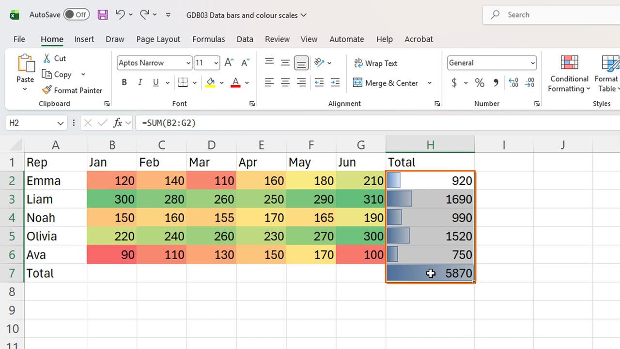
← Previous tutorial: Excel Slicers: Why Your SUM Total Never Changes
Next tutorial: An Excel Chart Title That Updates Itself →