Excel Slicers: Why Your SUM Total Never Changes
Add a slicer to a Table from the keyboard, then see why SUM ignores it and SUBTOTAL 109 follows it.
- Click to filter
- Make a Table
- Two totals
- Insert a slicer
- The SUM trap
Step by step
1. Click to filter
A slicer turns a dashboard into something anyone can click: one button, and the whole report shows one region. But one popular formula ignores it.
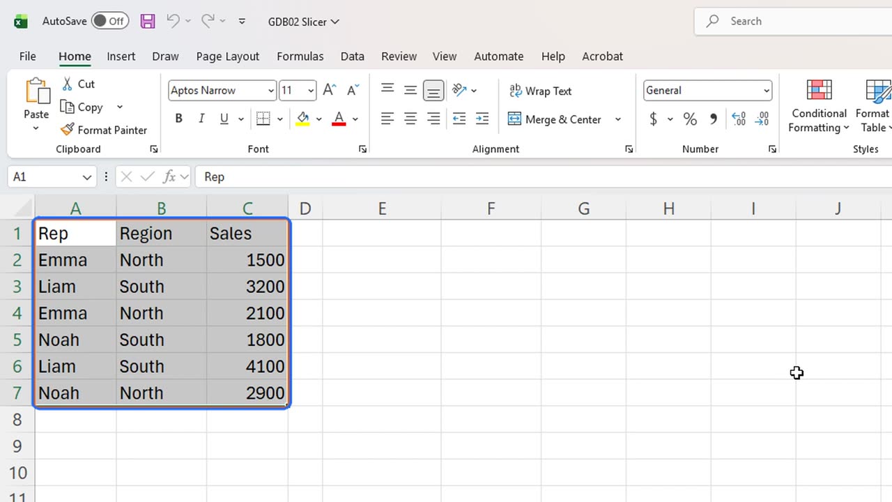
2. Make a Table
Slicers need a Table. Select the data and press Control and T.
Confirm the headers with Enter.
Shortcut: Ctrl + T
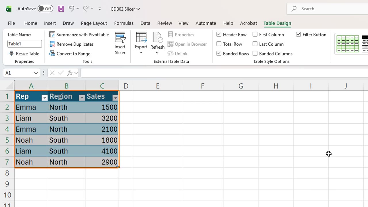
3. Two totals
Now two totals, side by side. In E1 type SUBTOTAL, and in F1 type SUM.
In E2, type SUBTOTAL, one hundred and nine, and the Sales column. Nine means sum, and the one in front means: skip the rows that are hidden.
In F2, a plain SUM of the same column. Both show fifteen thousand six hundred, for now.
=SUBTOTAL(109,Table1[Sales])=SUM(Table1[Sales])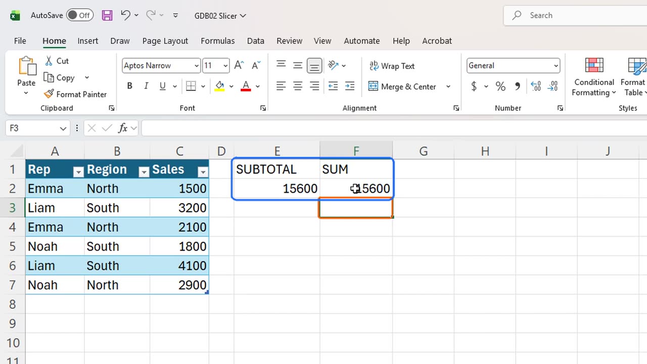
4. Insert a slicer
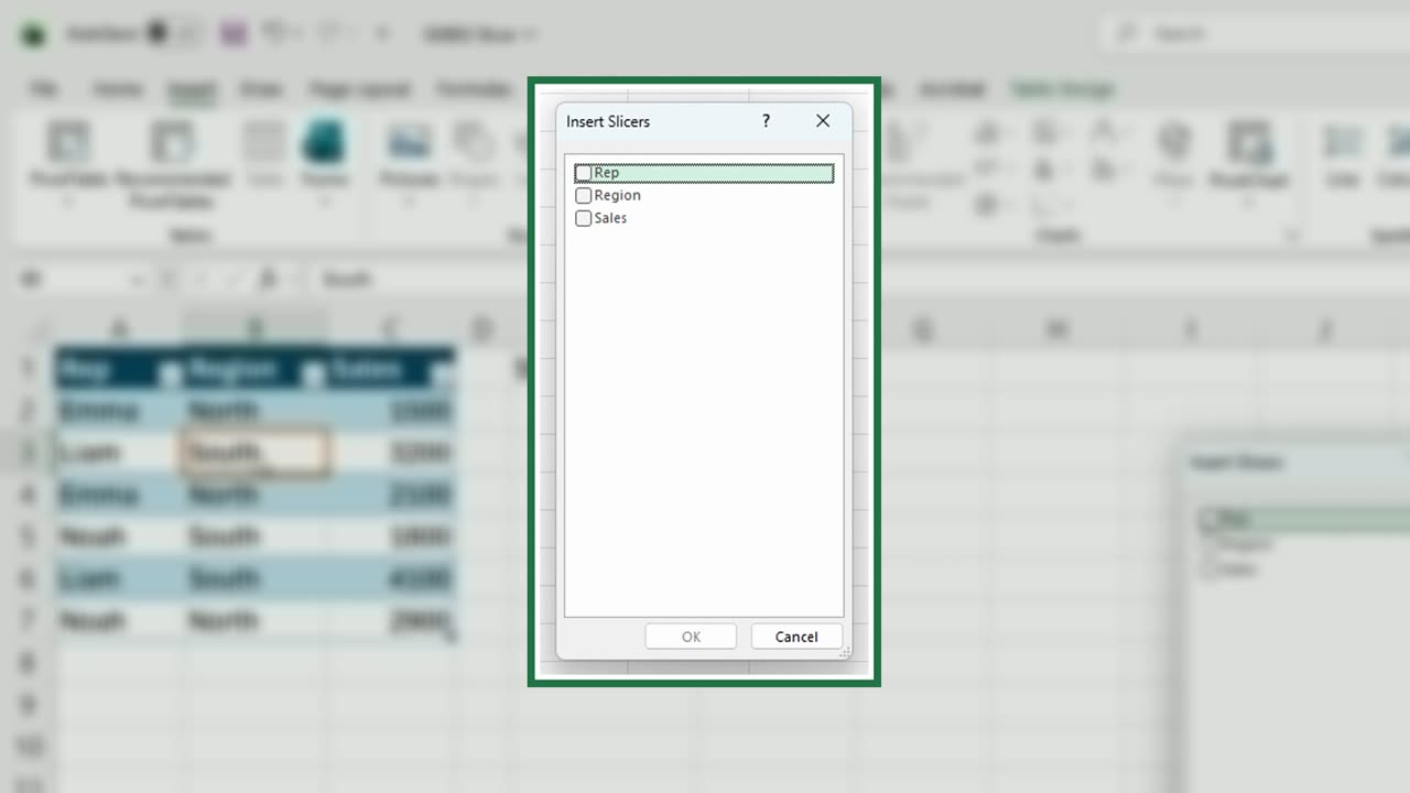
Now the slicer. Click inside the Table and press Alt, N, S, F. That is Insert, Slicer.
Excel lists every column. Press Down to reach Region, Space to tick it, and Enter.
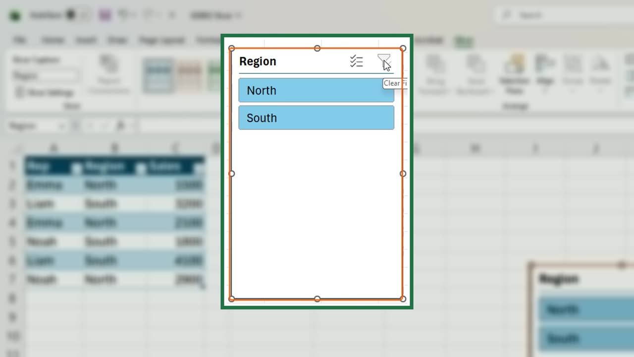
There it is: a box with one button for each region.
5. The SUM trap
Click North. The Table hides every South row at once.
Look at the totals. SUBTOTAL shows six thousand five hundred, only North. SUM still shows fifteen thousand six hundred, the hidden rows included.
That is the trap. A dashboard built on SUM looks interactive, but its numbers never move. Use SUBTOTAL, or AGGREGATE, for anything a slicer should control.
Click South, and SUBTOTAL follows again: nine thousand one hundred.
To show everything again, click the clear filter icon in the corner of the slicer.
Which field would you put on a slicer in your own report? Tell me in the comments.
← Previous tutorial: Build a Self-Updating Dashboard in Excel
Next tutorial: Turn a Grid of Numbers into a Picture in Excel →