Freeze Panes in Excel (Keep Headers Visible)
Freeze rows and columns, split windows and work with big sheets.
- Intro
- The problem
- Freeze the top row
- Freeze the first column
- Freeze both
- Unfreeze
- Recap
Step by step
1. Intro
Welcome back. Real sheets are often much bigger than your screen. In this lesson, you will keep the headers in view while you scroll, with Freeze Panes.
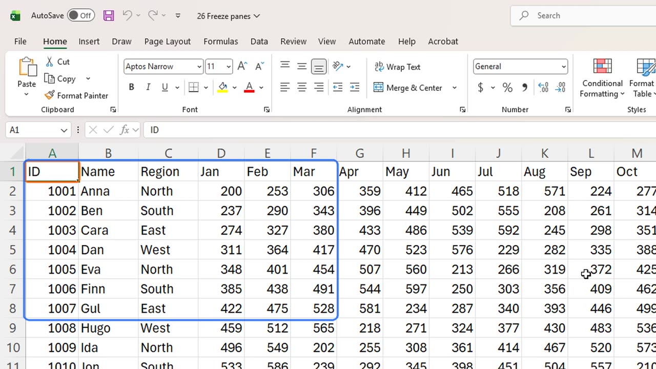
Here are thirty sales reps, with their sales for every month of the year.
2. The problem
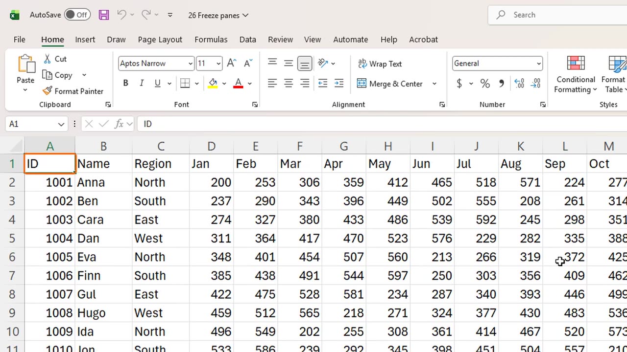
Watch what happens when we scroll down, with Page Down. The headers disappear. Which month is this column again?
Press Control and Home to go back to the top.
3. Freeze the top row
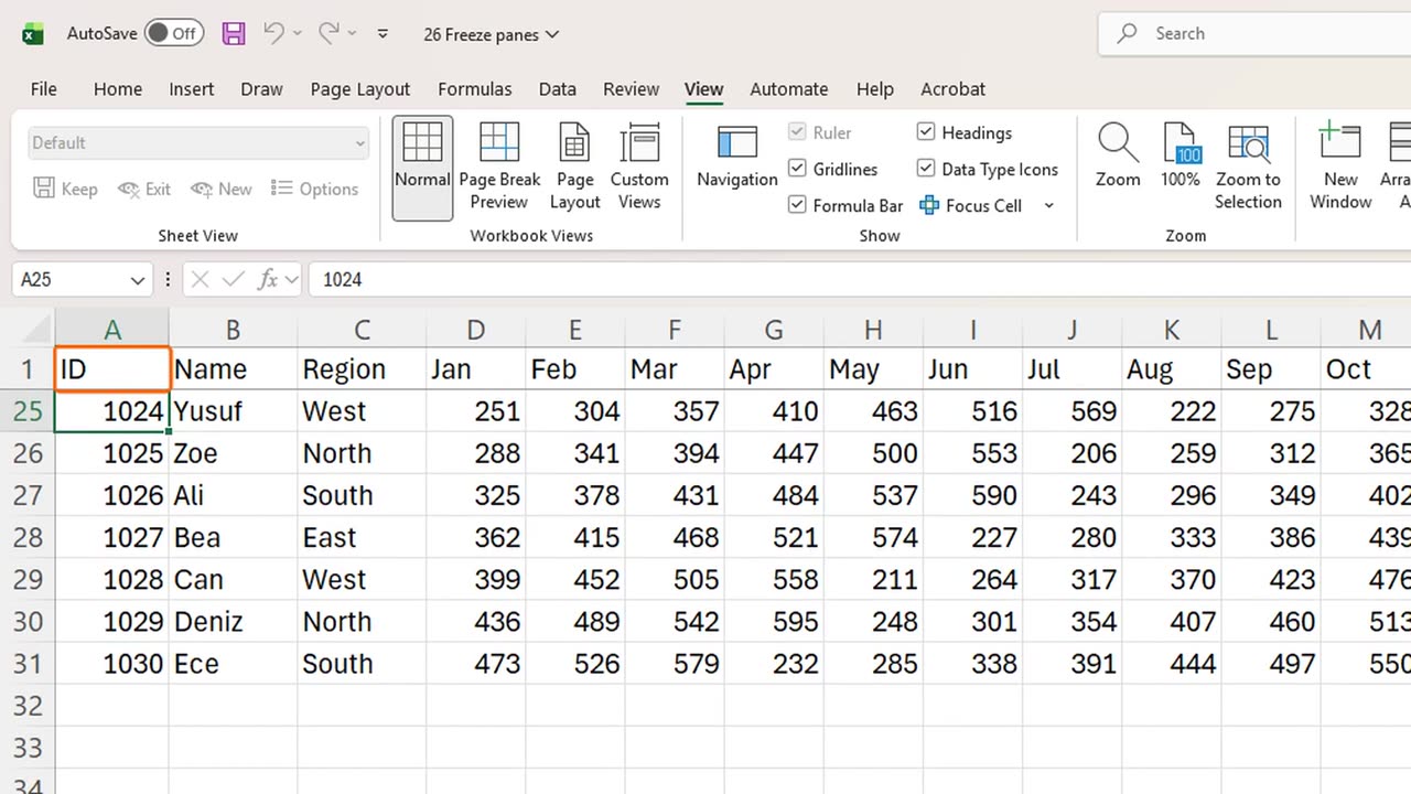
On the View tab, open Freeze Panes, and choose Freeze Top Row. The shortcut is Alt, W, F, R.
A thin line appears under row one. Now scroll down again. The headers stay at the top, and the rows move underneath them.
4. Freeze the first column
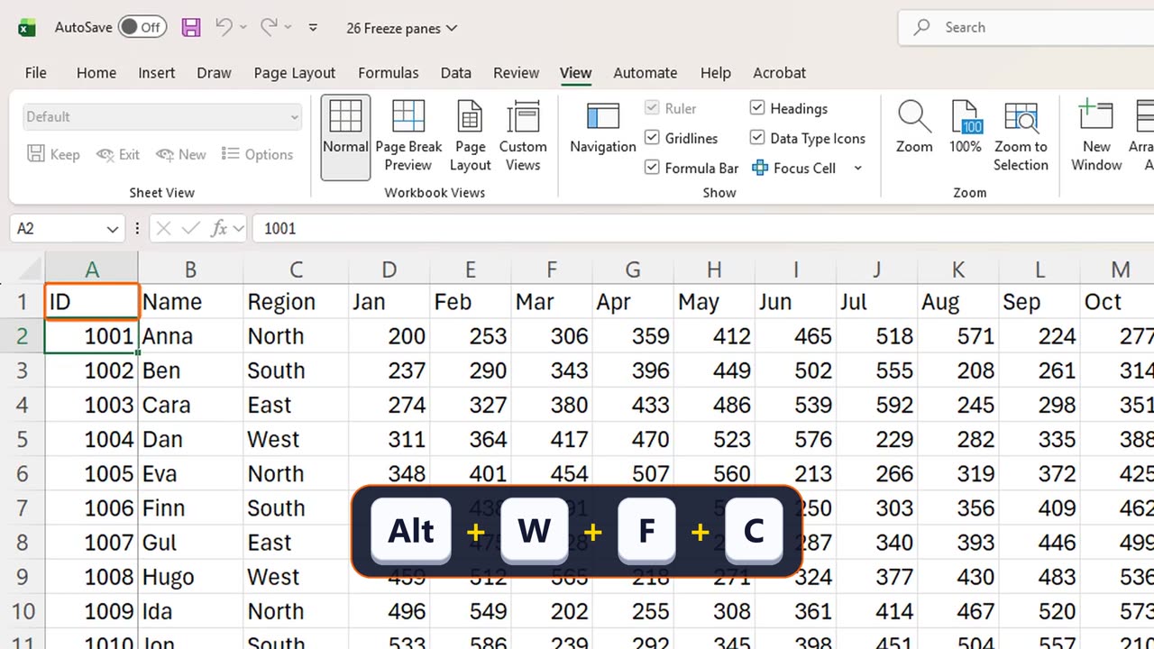
Now the other direction. Go back with Control Home, and scroll to the right with Alt and Page Down. This time the names disappear.
Freeze First Column, with Alt, W, F, C, keeps column A in place. But only one of these two works at a time.
5. Freeze both
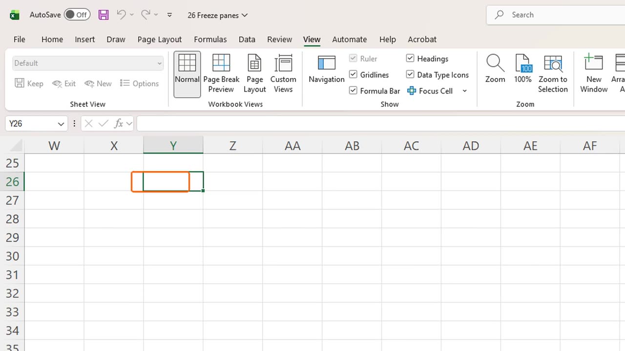
To keep both the header row and the name columns, use Freeze Panes itself. Click the first cell that should scroll. Here that is D2: everything above it and to its left will stay put.
Choose Freeze Panes, with Alt, W, F, F.
Scroll down, and to the right. Row one stays at the top, and the ID, name and region stay on the left. You always know whose number you are reading, and for which month.
6. Unfreeze
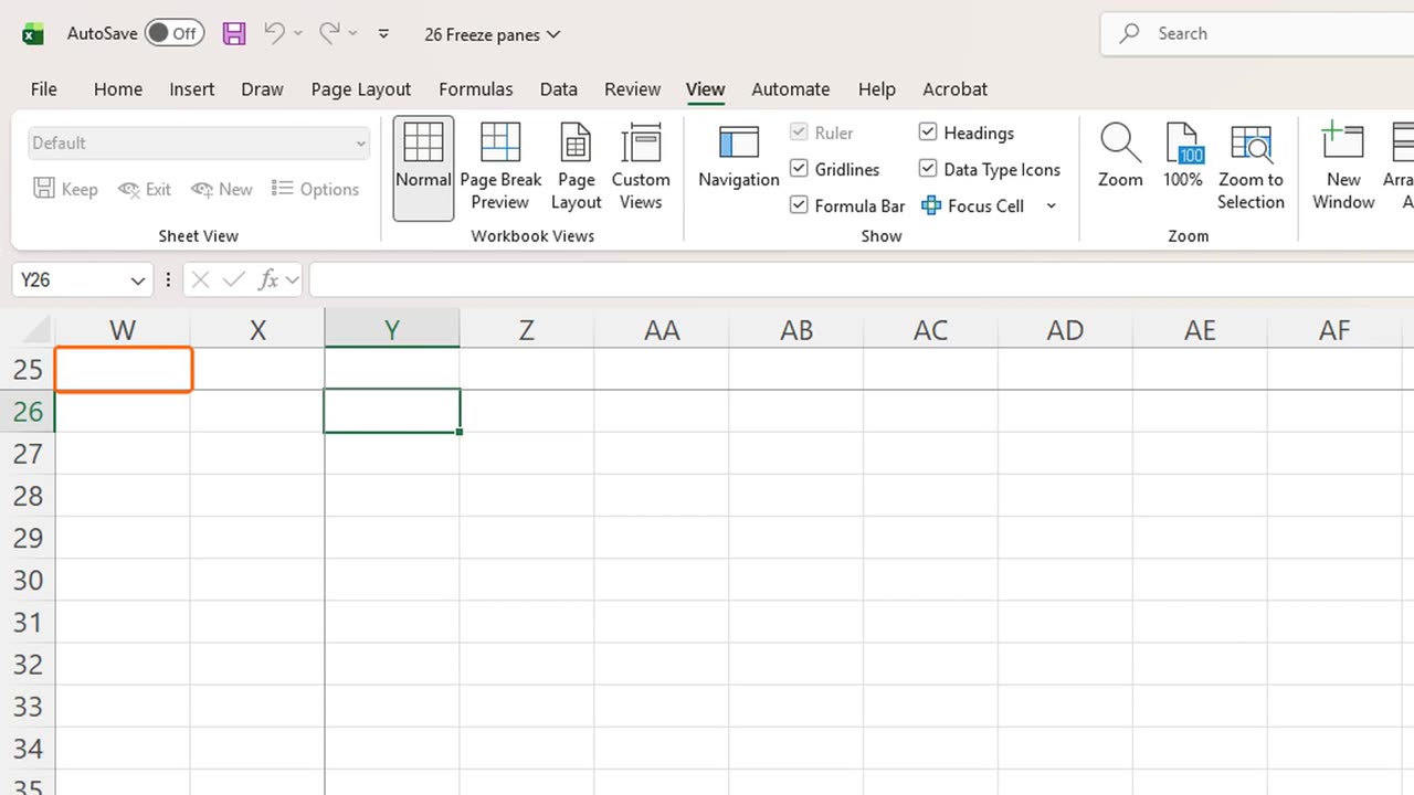
To undo it, open Freeze Panes again. The first choice is now called Unfreeze Panes.
A related tool is Split, also on the View tab. It divides the window into parts that scroll on their own, so you can compare the top and the bottom of a long list.
7. Recap
Let's recap. Freeze Top Row keeps the headers, Freeze First Column keeps the names, and Freeze Panes keeps everything above and to the left of the cell you click.
That completes Module 3, on working with data. In the next module, you will turn your numbers into charts and PivotTables.
If there is something you want to learn next, write it in the comments. Your requests decide what we teach in the next tutorials. Thanks for watching, and see you in the next one.
← Previous tutorial: Excel Flash Fill (Ctrl + E): Auto-Format Data
Next tutorial: How to Make a Chart in Excel (Column, Line, Pie) →