How to Make a Chart in Excel (Column, Line, Pie)
Create your first chart and choose the right type.
- Numbers to picture
- Column chart
- Switch to a line
- Pie chart
- The pie trap
- Recap
Step by step
1. Numbers to picture
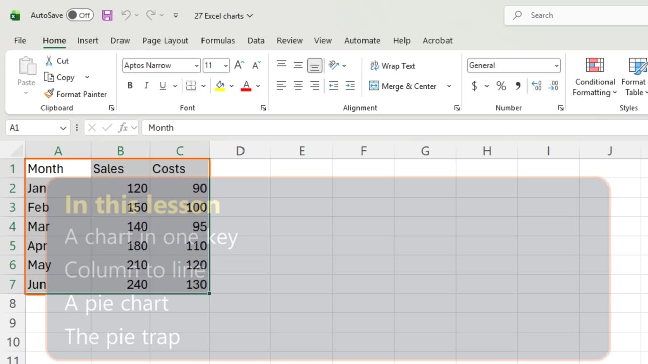
Six months of sales and costs. As numbers they say very little. As a chart, the story jumps out in one second.
You will make a column chart, switch it to a line, and build a pie, plus the one mistake that breaks every pie.
2. Column chart
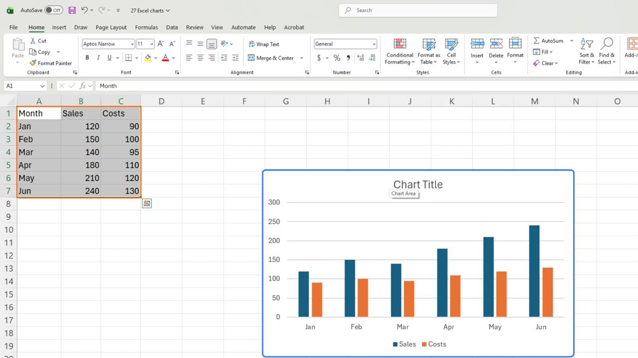
Select the data, headers included. Then press Alt and F1.
That is a column chart. Each month gets two bars, blue for sales and orange for costs, and the legend underneath says which is which.
Column charts are best for comparing amounts side by side. June clearly beats January.
3. Switch to a line
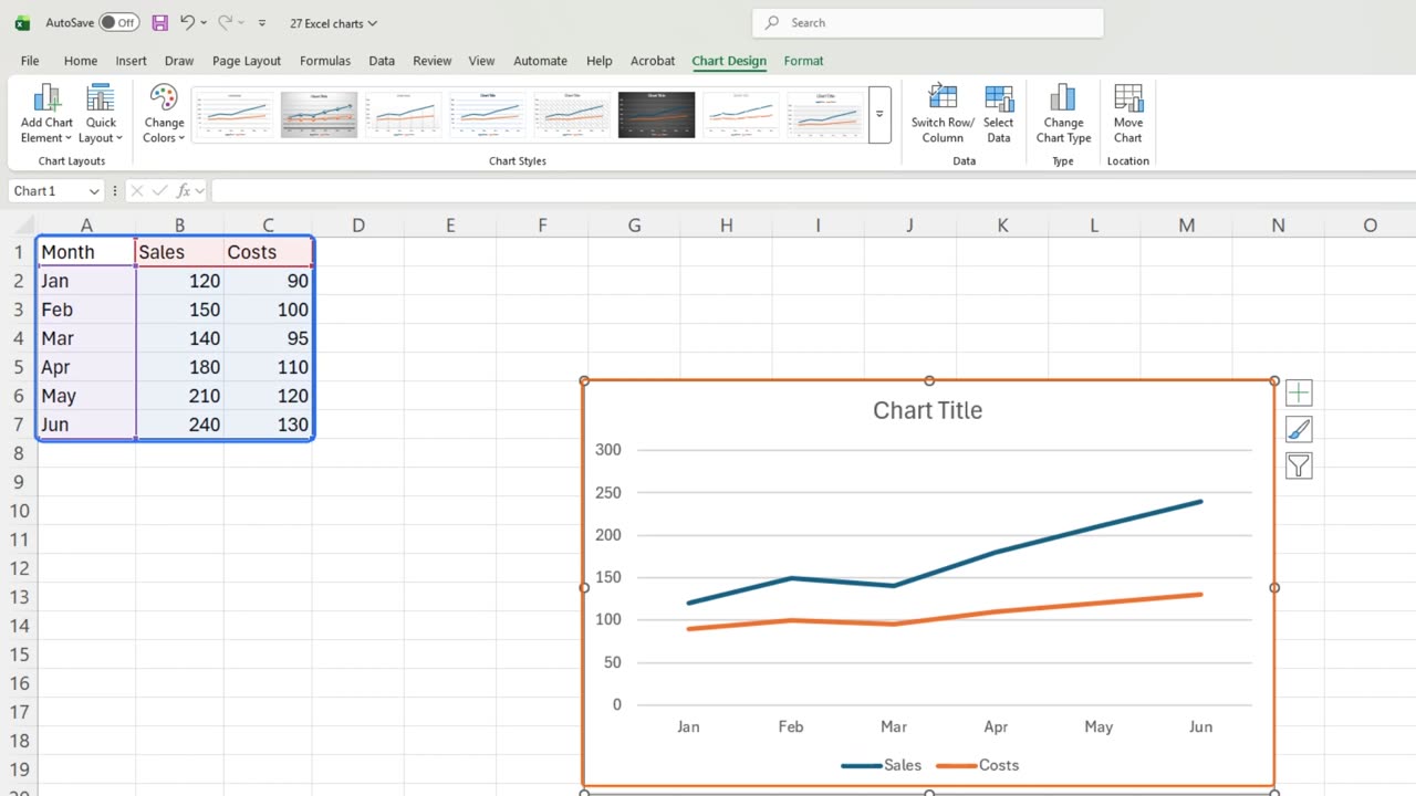
But this data is a trend over time, and a line shows a trend better. With the chart selected, open Change Chart Type: Alt, J, C, C.
Choose Line on the left, and press Enter.
Same data, new picture. Both lines climb, and the gap between them, your profit, grows every month.
Quick pause: if this is clear so far, a like really helps the channel. The next part is where most pie charts go wrong.
4. Pie chart
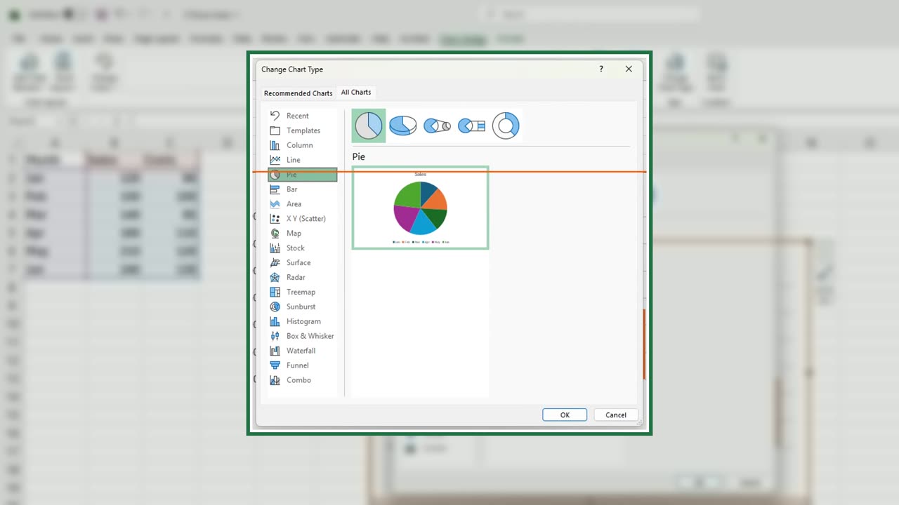
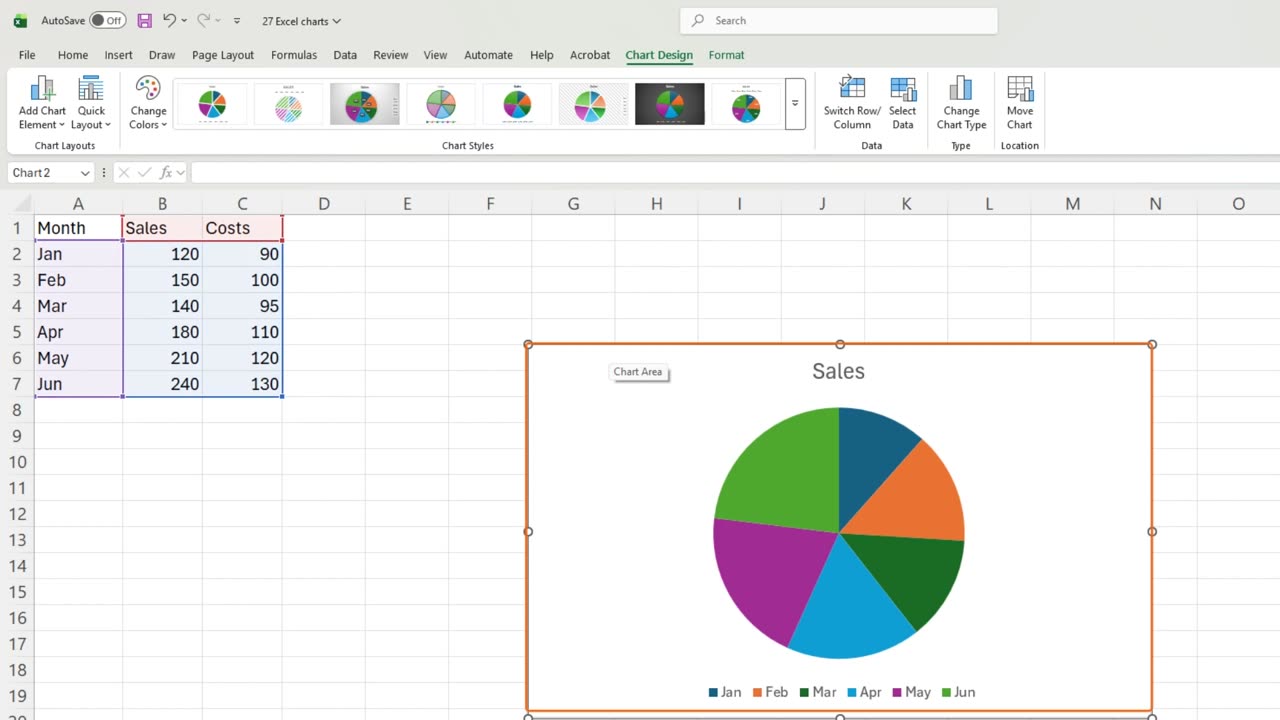
Now a pie. Click a cell outside the chart, select the data again, press Alt and F1, and switch the type to Pie the same way.
5. The pie trap
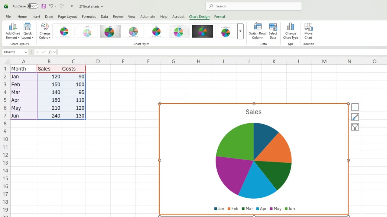
Here is the trap. The pie shows only sales. Costs vanished without a warning, because a pie can show just one series.
So use a pie only for parts of one whole, like each month's share of the half year, and keep it to a few slices.
6. Recap
Recap: Alt and F1 makes a chart, Change Chart Type switches it, columns compare, lines show trends, and a pie shows one series only.
In the next lesson, you will format a chart like a pro: titles, labels and colors.
Which chart type do you use most at work? Tell me in the comments.
← Previous tutorial: Freeze Panes in Excel (Keep Headers Visible)
Next tutorial: Format Excel Charts Like a Pro (Titles, Labels, Colors) →