Build a Self-Updating Dashboard in Excel
Turn a list of sales into a dashboard with a total, a region summary, in-cell bars and a top seller, all updating by themselves.
- The goal
- Make a Table
- The first KPI
- Sales by region
- In-cell bars
- Top performer
- The test
- The spill trap
Step by step
1. The goal
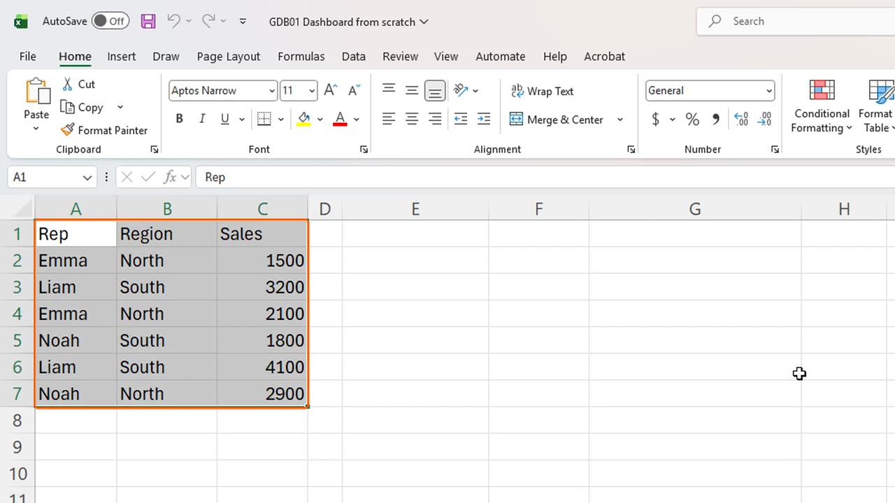
A table of sales numbers is accurate, but nobody wants to read it. Here is how to turn it into a dashboard that keeps itself up to date.
2. Make a Table
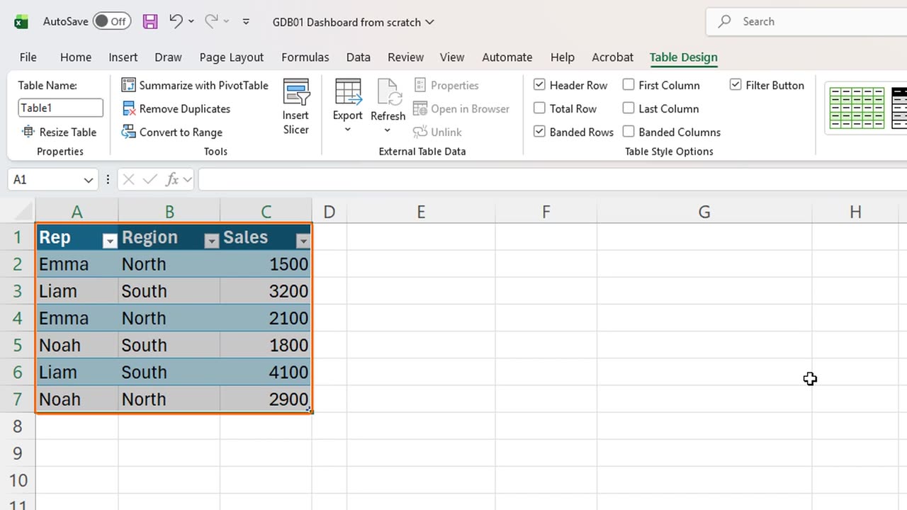
The whole dashboard rests on one habit: turn the list into a Table first. Select the data and press Control and T.
Excel asks whether the table has headers. It does, so press Enter.
A Table grows by itself when you add rows, and every formula that points at it grows too. That is the secret behind a dashboard that never needs repairs.
Shortcut: Ctrl + T
3. The first KPI
Now the first number everyone asks for: total revenue. In E2, type the label Total Revenue.
In F2, type equals SUM, open the bracket, and click through to the Sales column of the Table. Excel writes the column name for you.
Fifteen thousand six hundred. Because the formula uses the column name instead of cell addresses, it will include every future row.
=SUM(Table1[Sales])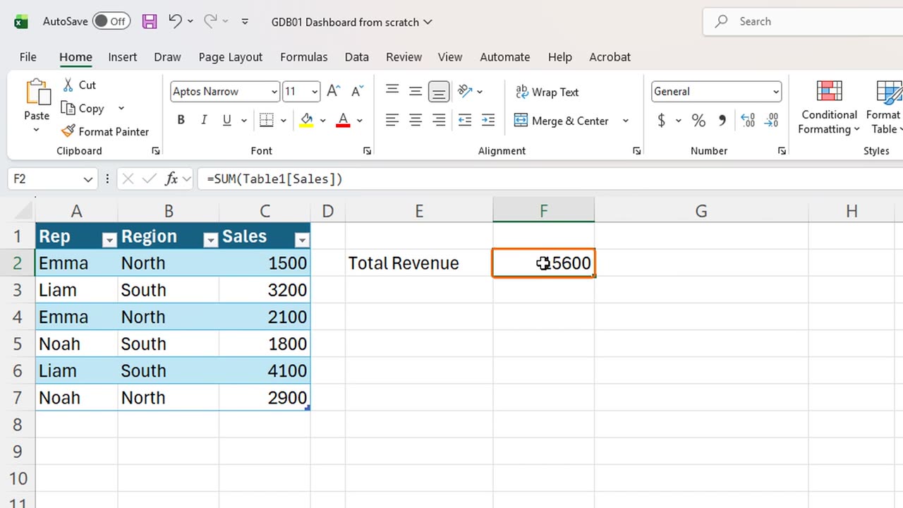
4. Sales by region
Next, sales by region. In E4, type Region, then Tab, and Sales.
Instead of typing the region names, let a formula find them. In E5, type equals UNIQUE of the Region column.
One formula, and the list of regions spills down by itself: North and South. If a new region ever appears in the data, it joins the list.
Beside it, in F5, add up the sales for each region. Type equals SUMIFS, the Sales column, the Region column, then E5 followed by a hash sign.
The hash sign means the whole spilled list. So this one formula fills both cells: six thousand five hundred for North, nine thousand one hundred for South.
=UNIQUE(Table1[Region])=SUMIFS(Table1[Sales],Table1[Region],E5#)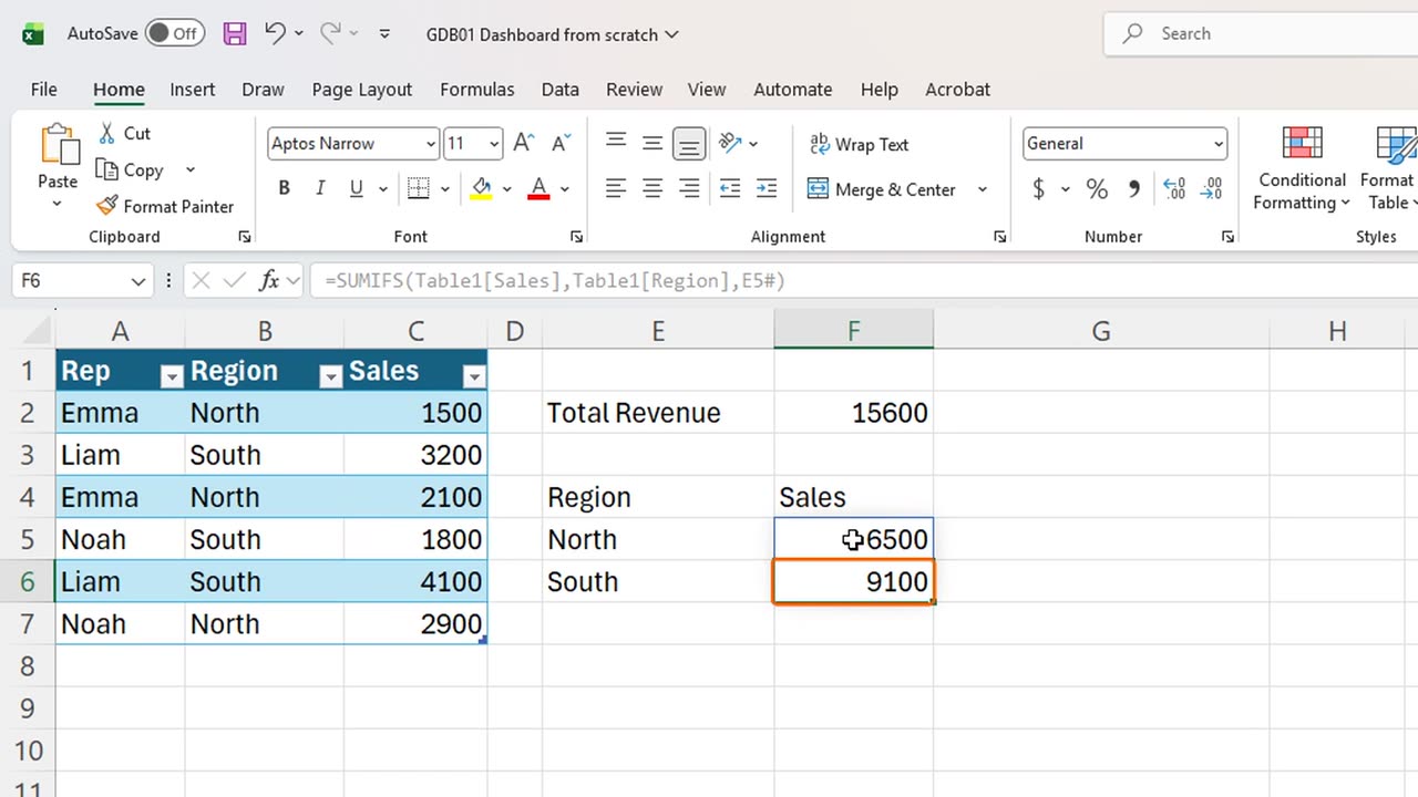
5. In-cell bars
Dashboards need visuals, and you do not need a chart for that. In G4, type Trend. In G5, repeat a bar character with REPT, one bar for every three hundred in sales.
Copy the formula down by dragging the fill handle, and every region gets a bar that is perfectly in proportion to its sales.
=REPT("|",F5/300)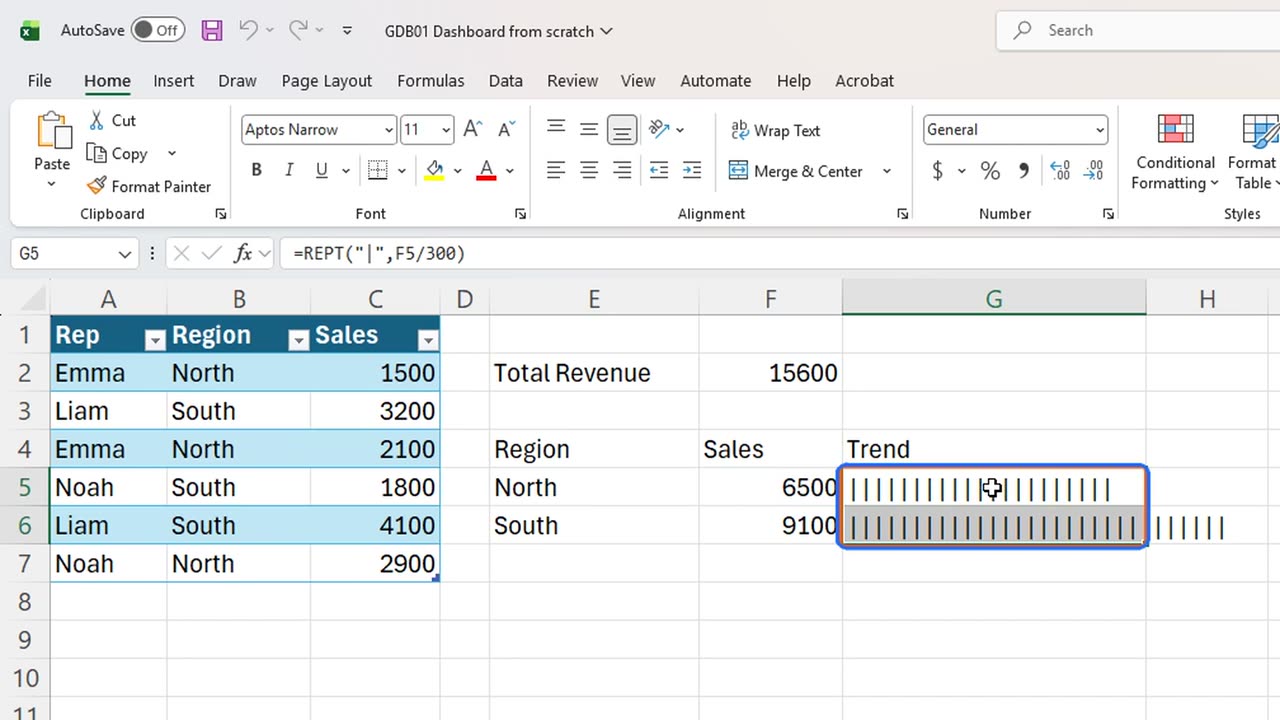
6. Top performer
One more insight: who is the top seller? In E8, type Top Rep. In F8, nest MAX inside XLOOKUP, so Excel finds the biggest sale and returns the name next to it.
=XLOOKUP(MAX(Table1[Sales]),Table1[Sales],Table1[Rep])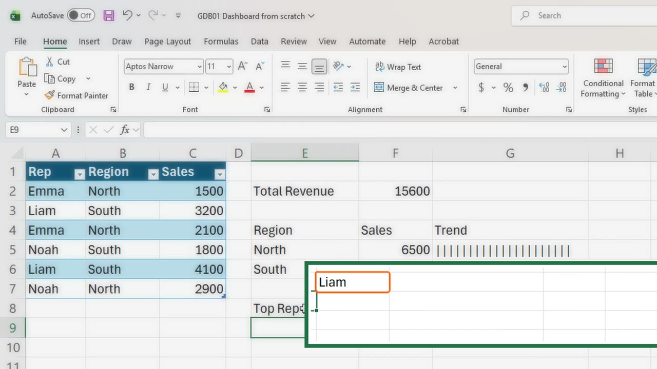
7. The test
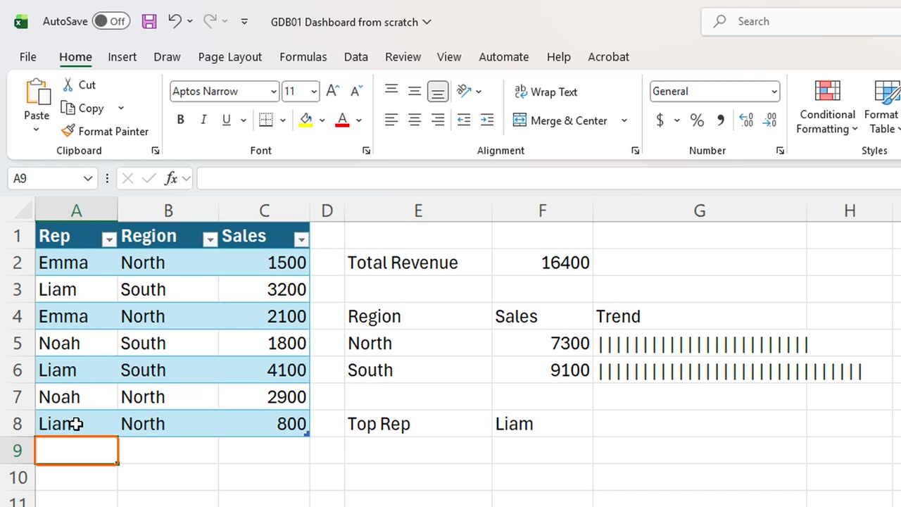
Liam, with a single sale of four thousand one hundred. Now the real test: add a new row under the Table.
Type Liam, North, and eight hundred, pressing Tab between the cells.
The Table swallows the new row, and the dashboard follows: the total is sixteen thousand four hundred, and North is now seven thousand three hundred. Nothing was edited by hand.
8. The spill trap
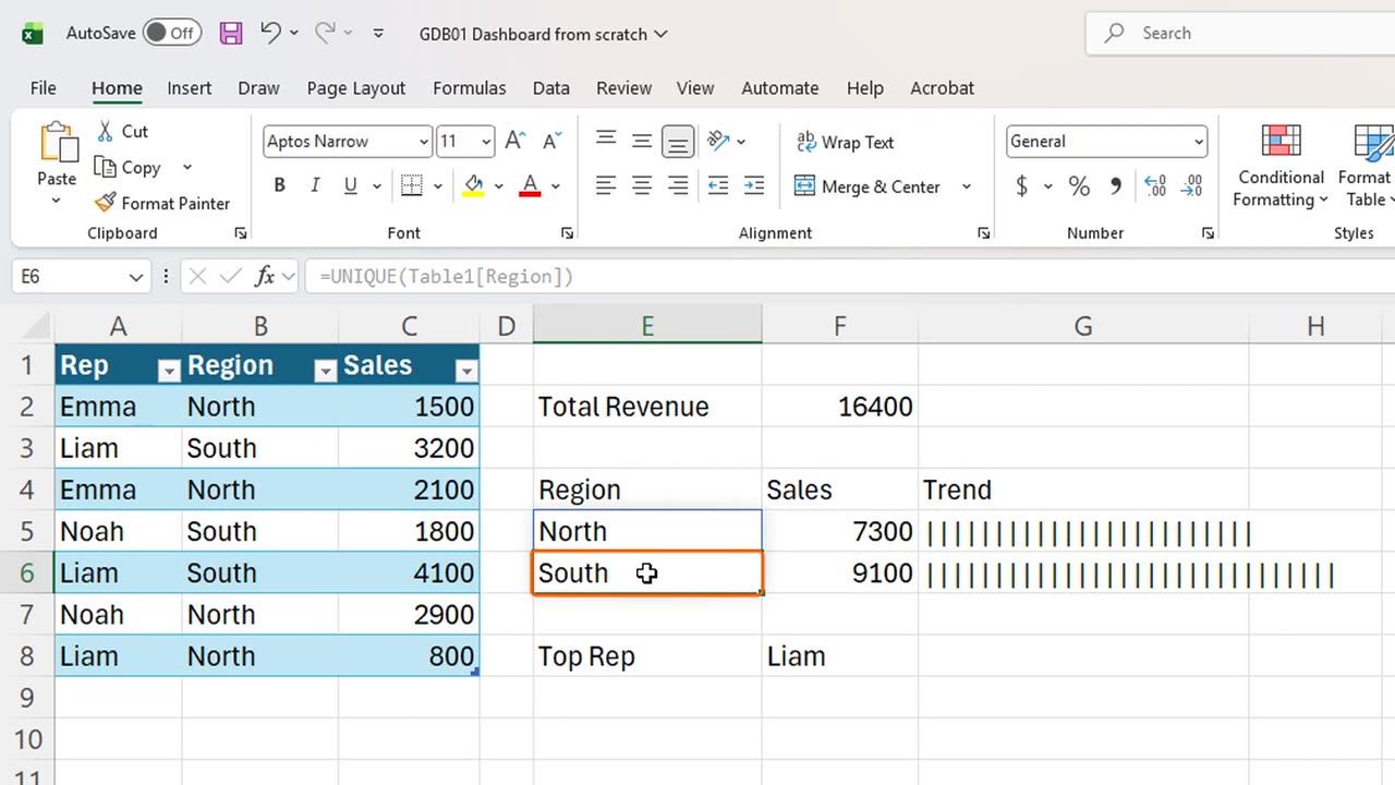
Here is the trap. Dynamic arrays need empty room to spill. Type anything in E6, just under North, and watch E5.
A spill error. Excel will not overwrite your cell. The fix is simple: delete the blocking entry, and the list returns by itself.
Which number would you add to this dashboard first? Write it in the comments, and I will build it.
← Previous tutorial: Clean Messy Data with Copilot in Excel
Next tutorial: Excel Slicers: Why Your SUM Total Never Changes →