Format Excel Charts Like a Pro (Titles, Labels, Colors)
Titles, data labels, axes, colors and templates.
- Default to pro
- Title
- Data labels
- Less clutter
- A calmer style
- The title trap
- Recap
Step by step
1. Default to pro
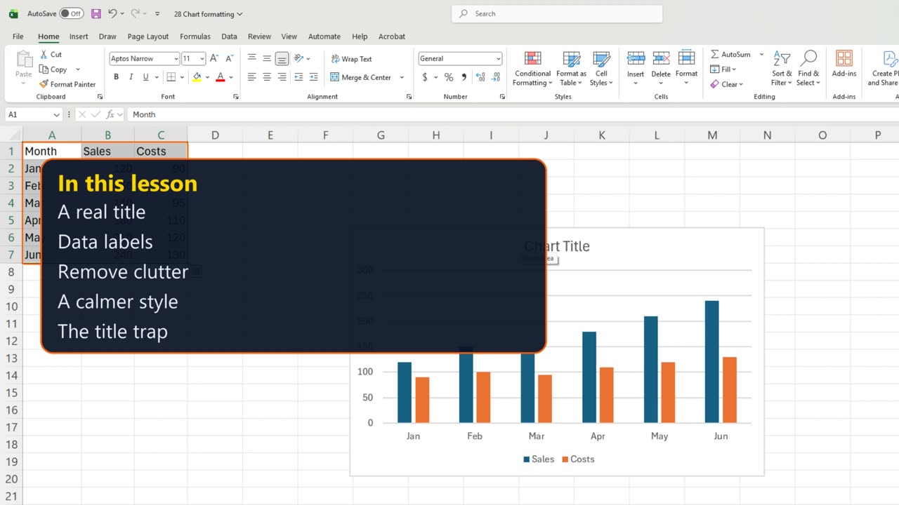
A default chart works, but nobody reads it. Four quick changes turn it into a chart people understand at a glance.
A real title, numbers on the bars, less clutter, and a calmer style.
2. Title
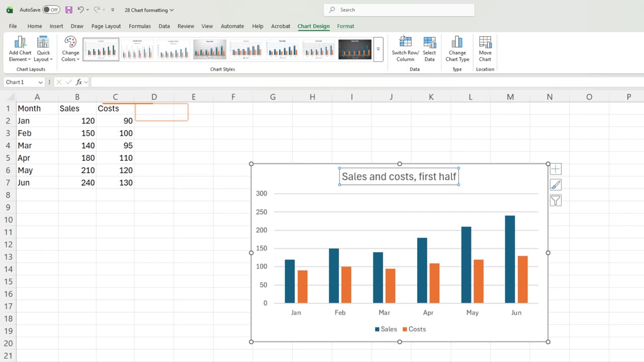
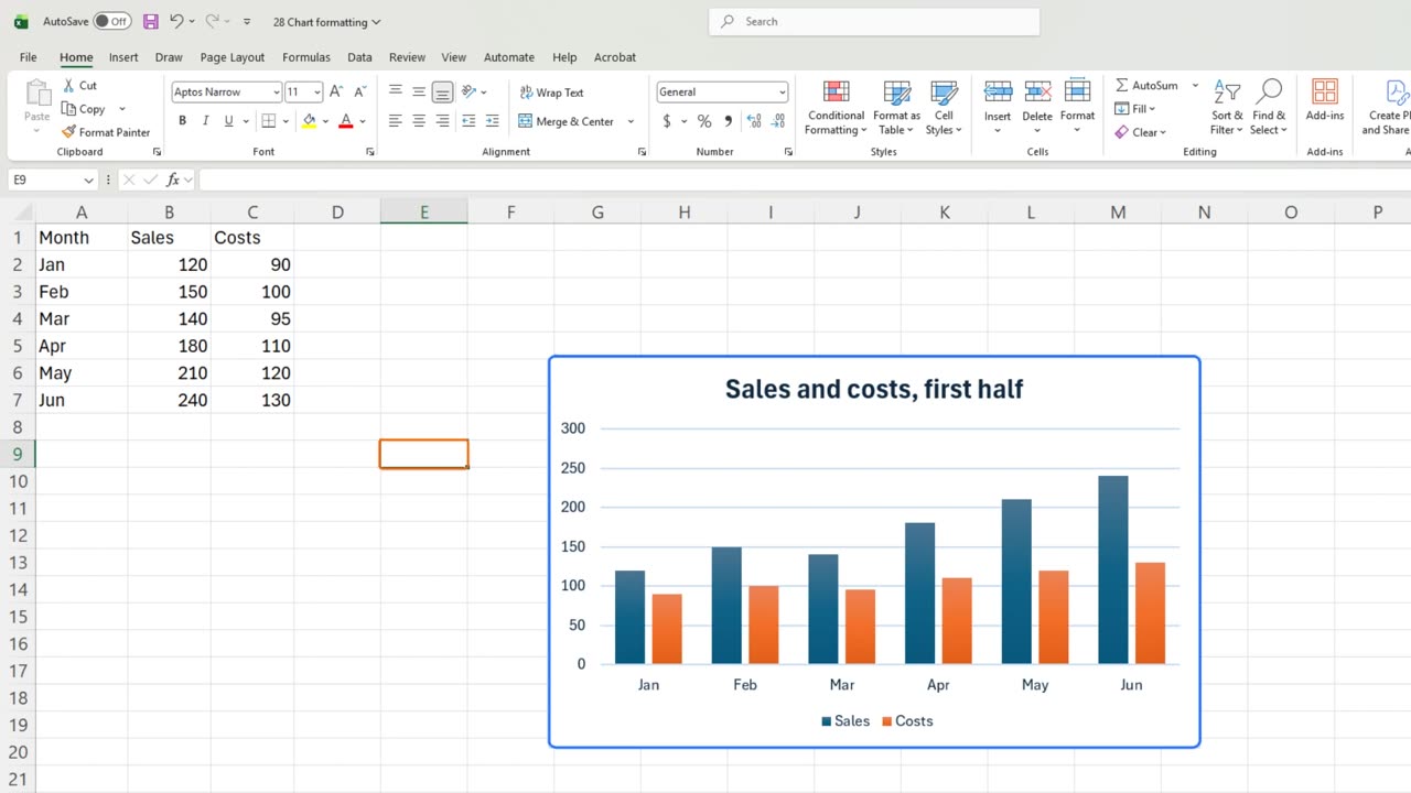
Start with the title. Chart Title says nothing. Click it once, type Sales and costs, first half, and press Enter.
3. Data labels
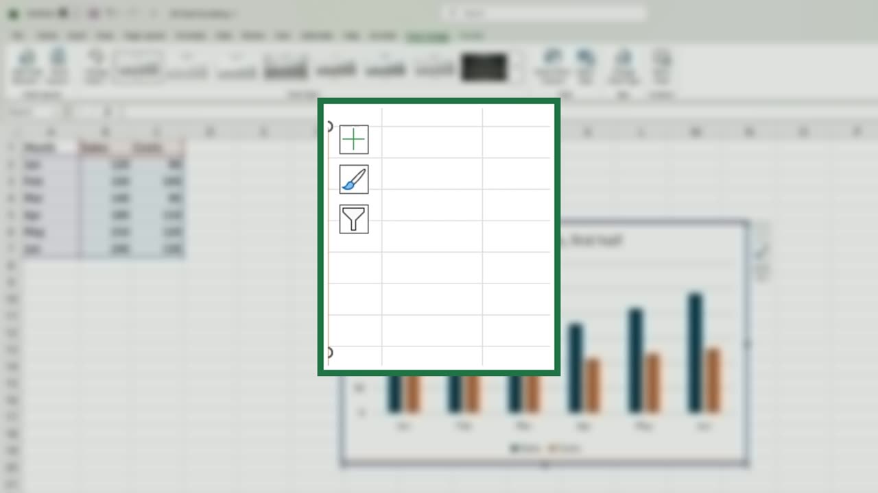
Next, the exact numbers. Click the plus button beside the chart. These are the chart elements.
Tick Data Labels. Every bar now shows its value, so nobody has to guess from the axis.
4. Less clutter
With labels on, the gridlines are clutter. Untick Gridlines.
Quick pause: if your charts already look better, a like really helps the channel. Next comes the style, and then the trap.
5. A calmer style
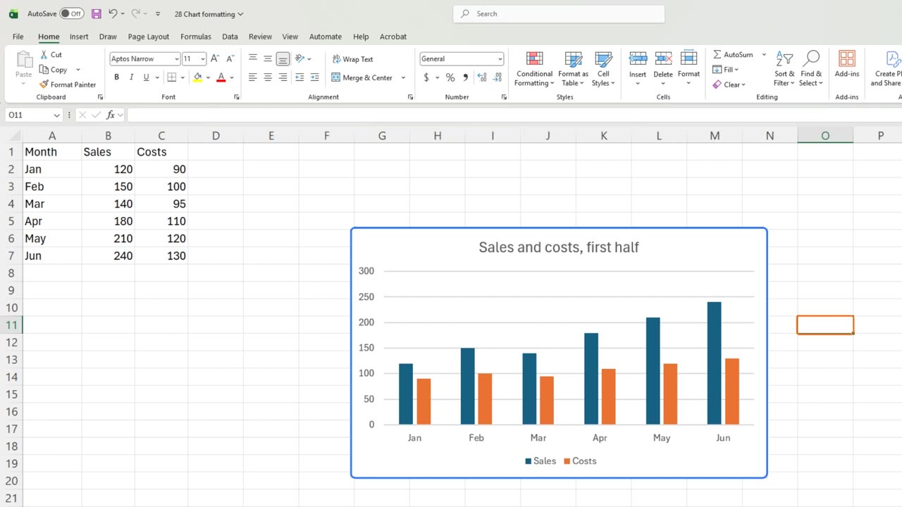
Now the look. With the chart selected, open Chart Design and pick a calmer style from the gallery.
Click any cell. Clear title, exact labels, no grid, a calm style. This chart reads in two seconds.
6. The title trap
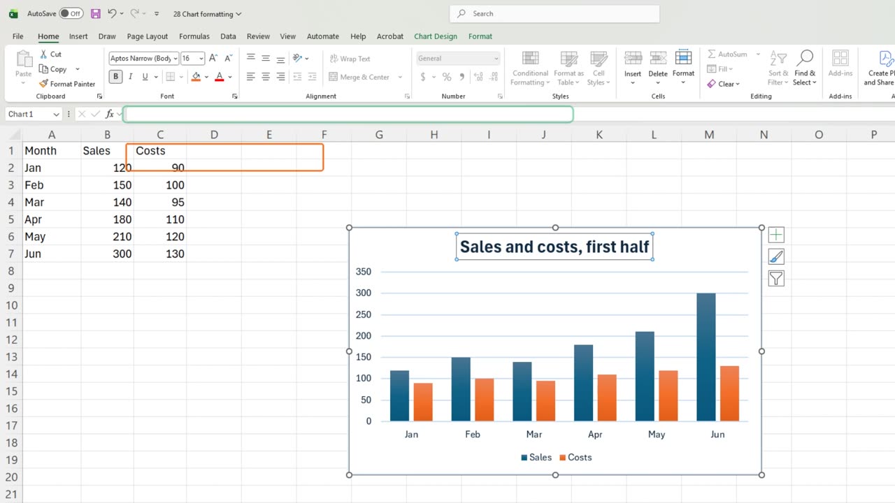
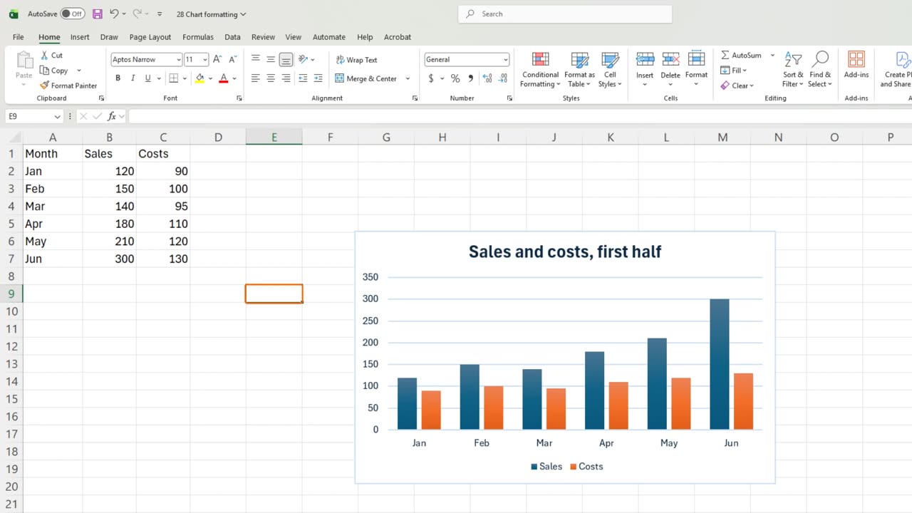
Now the trap. Change June's sales to three hundred. The bar and its label update by themselves.
But the title is typed text. If it should say a total or a month, it will never update. Link a title to a cell instead, and it changes with the data.
7. Recap
Recap: a clear title, data labels, no gridlines, one calm style, and titles linked to cells when they show numbers.
In the next lesson, you will put tiny charts inside cells with sparklines.
What is the first thing you change on every new chart? Tell me in the comments.
← Previous tutorial: How to Make a Chart in Excel (Column, Line, Pie)
Next tutorial: Excel Sparklines: Tiny Charts in a Cell →