Excel Text to Columns: Split Data into Columns
Split full names, dates and imported data with Text to Columns.
- Intro
- Split by space
- Split by another character
- Recap
Step by step
1. Intro
Welcome back. Data often arrives with several pieces in one cell: a full name, or a code with parts. In this lesson, you will split one column into several, with Text to Columns.
2. Split by space
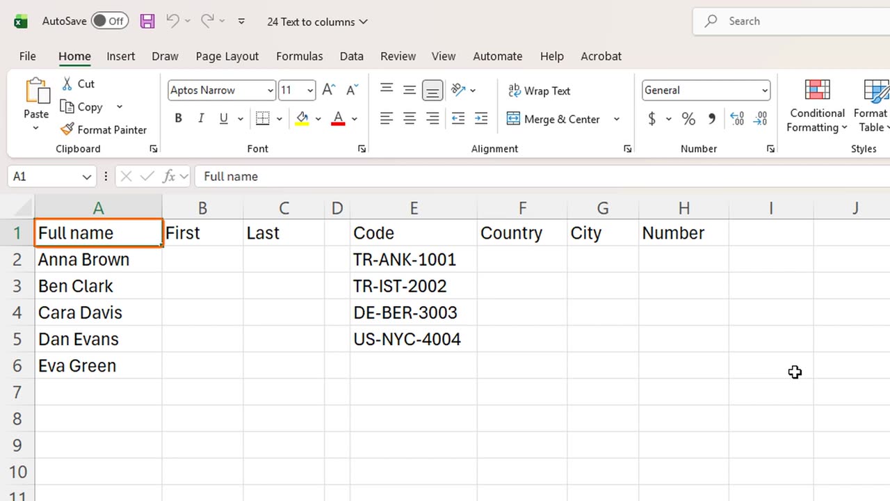
Here, column A has full names. We want the first name in column B and the last name in column C.
Select the names, A2 to A6. On the Data tab, choose Text to Columns, with Alt, A, E. A wizard with three steps opens.
Step one asks how the data is separated. Delimited is already chosen, which means a character, such as a space or a comma, separates the parts. Click Next.
In step two, tick Space. The preview below already shows the names in two columns. Click Next.
Step three is important. By default, the result replaces the original names. To keep them, set the Destination to B2. Then click Finish.
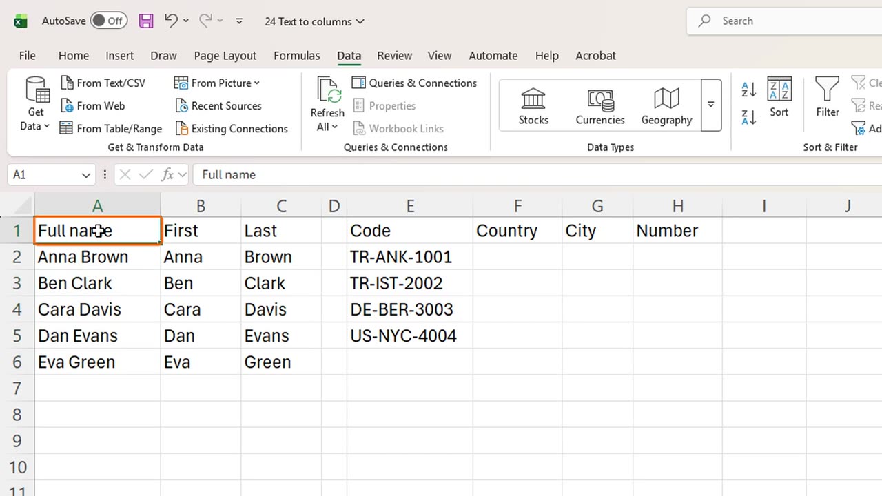
The first names are now in B and the last names in C, and the full names are still in A.
3. Split by another character
A second example. Column E has product codes, made of a country, a city and a number, separated by dashes.
Select E2 to E5, and open Text to Columns again. Click Next.
This time, untick Space, tick Other, and type a dash in the small box next to it. Click Next.
Set the Destination to F2, and click Finish.
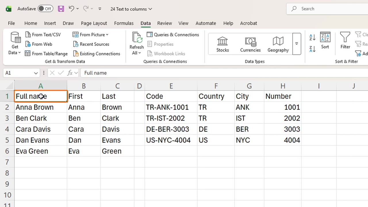
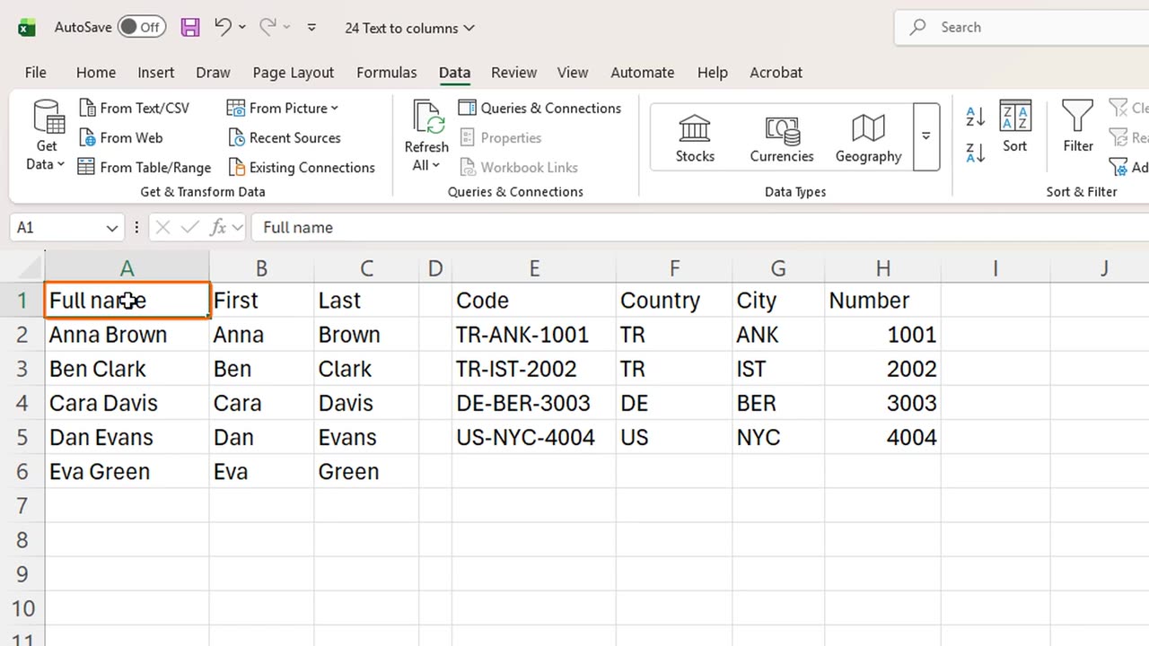
Each code is split into three columns. Notice that the number keeps working as a number, so you can add it up or sort it.
One warning: Text to Columns writes over any cells in its way, without asking first. Always check that the columns on the right are empty, or choose an empty destination.
4. Recap
Let's recap. Text to Columns splits one column by a space, a comma, a dash or any other character. Use the Destination box to keep your original data.
In the next lesson, you will meet Flash Fill, which splits and joins data just from one example.
If there is something you want to learn next, write it in the comments. Your requests decide what we teach in the next tutorials. Thanks for watching, and see you in the next one.
← Previous tutorial: Conditional Formatting in Excel (Highlight Cells Automatically)
Next tutorial: Excel Flash Fill (Ctrl + E): Auto-Format Data →