Conditional Formatting in Excel (Highlight Cells Automatically)
Highlight rules, data bars and color scales.
- Intro
- Highlight a limit
- Data bars
- Color scales
- Clear rules
- Recap
Step by step
1. Intro
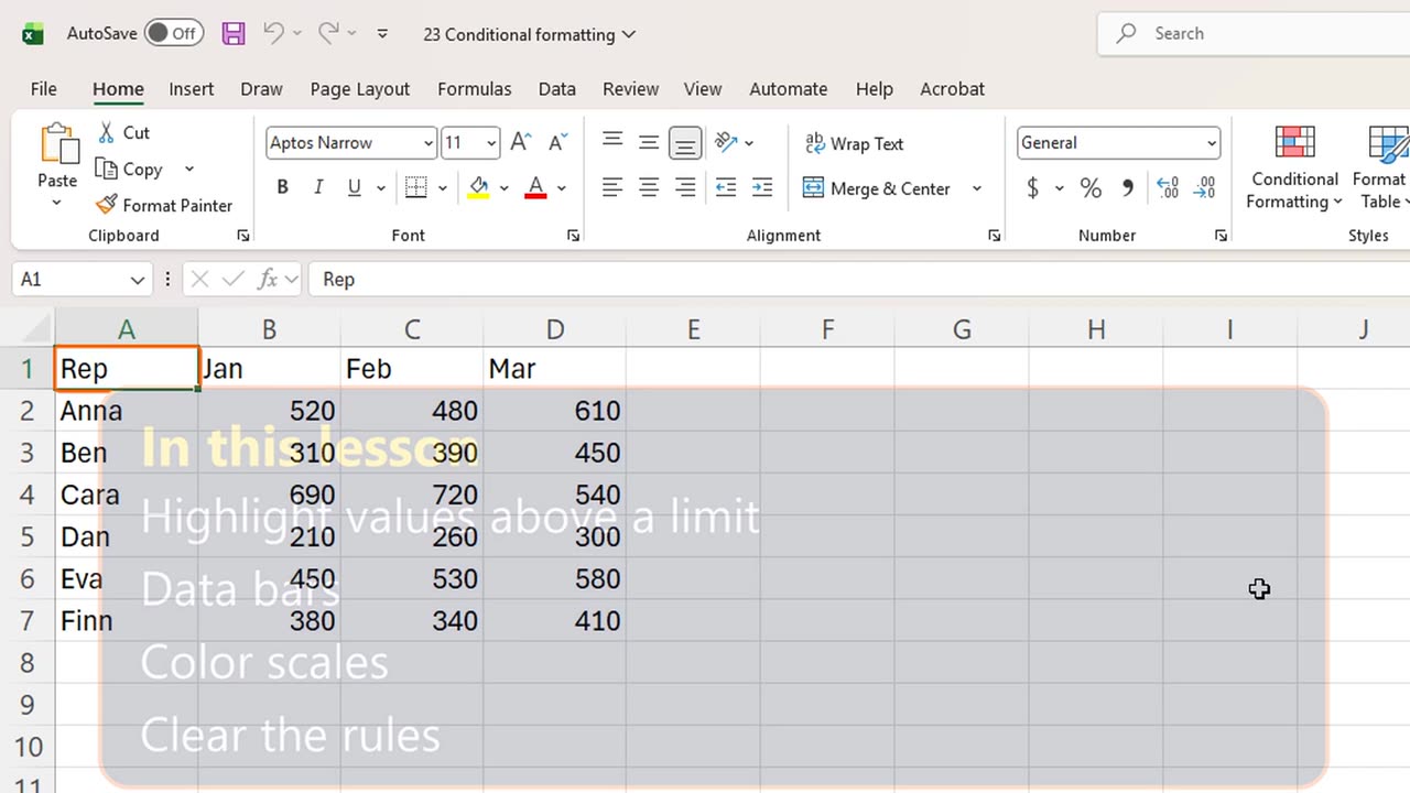
Welcome back. In this lesson, you will make Excel color your cells automatically, so the important numbers jump out at you.
This is called Conditional Formatting: the format depends on the value. When the value changes, the color changes with it.
2. Highlight a limit
Here are monthly sales for six reps, from January to March.
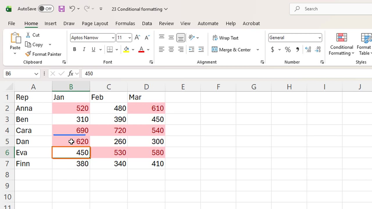
Let's highlight every month above five hundred. Select B2 to D7. On the Home tab, open Conditional Formatting, Highlight Cells Rules, Greater Than.
Type five hundred, and press Enter to accept the light red fill.
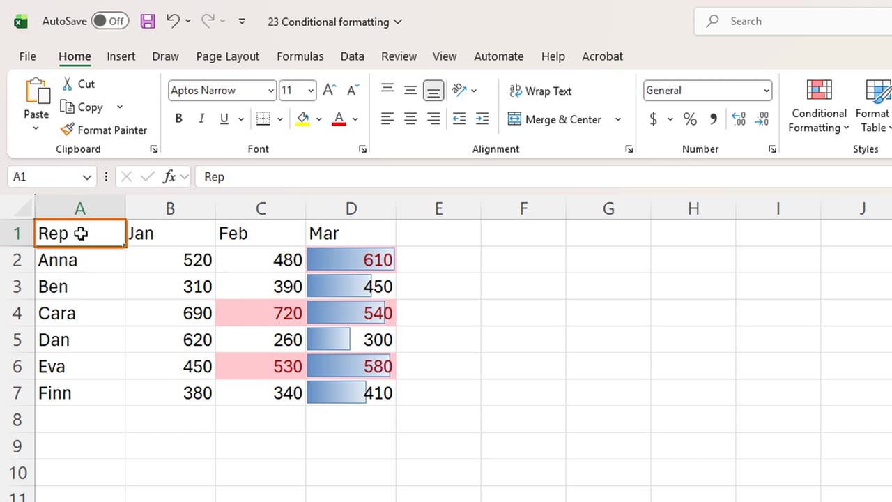
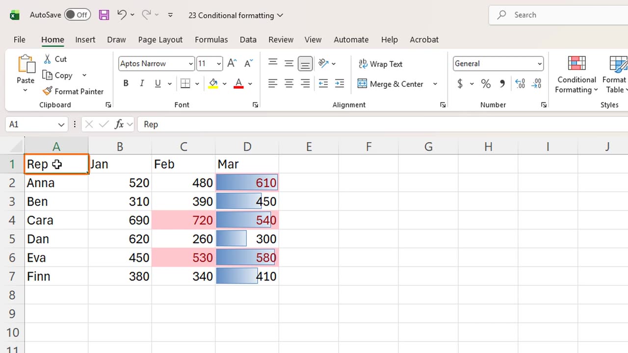
Every value above five hundred is now red. You can read the strong months at a glance, without checking each number.
The rule follows the value. Change Dan's January sales to six hundred and twenty. As soon as you press Enter, the cell turns red.
3. Data bars
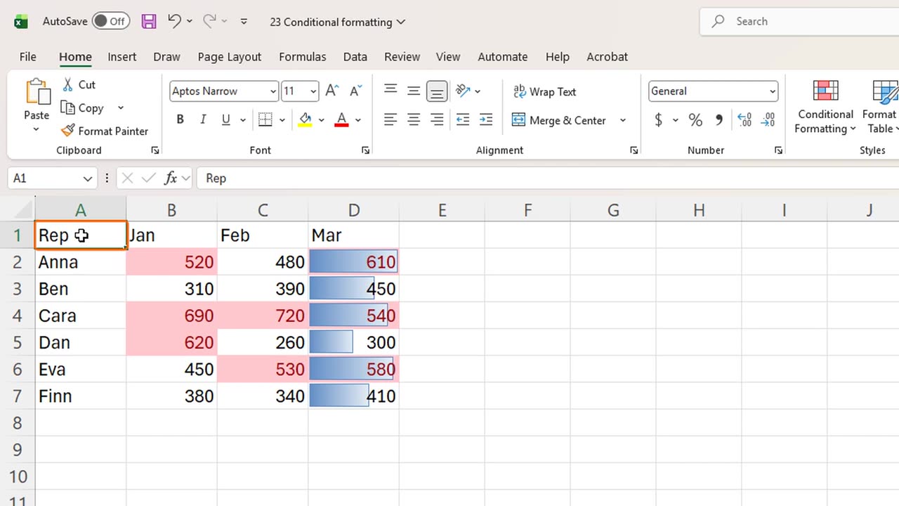
Next, data bars. Select the March numbers, D2 to D7. Open Conditional Formatting, Data Bars, and choose the first blue bar.
Each cell now holds a small bar chart. The longer the bar, the bigger the number. It is a chart, right inside your table.
4. Color scales
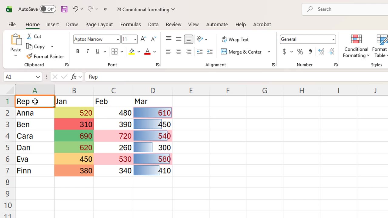
Color scales work the same way. Select the January numbers, B2 to B7, open Conditional Formatting, Color Scales, and pick the first one.
Green for the highest, red for the lowest, and shades in between. Color scales are great for spotting patterns in big tables.
5. Clear rules
Too many colors make a sheet hard to read, so use one or two rules at a time. To remove a rule, select its cells, and choose Clear Rules, Clear Rules from Selected Cells.
The color scale is gone, and the other rules are still there. Manage Rules, in the same menu, lists every rule on the sheet, if you ever need to edit one.
6. Recap
Let's recap. Highlight Cells Rules color values above or below a limit. Data bars and color scales compare numbers visually. And the colors update by themselves when the values change.
In the next lesson, you will split one column into several, with Text to Columns.
If there is something you want to learn next, write it in the comments. Your requests decide what we teach in the next tutorials. Thanks for watching, and see you in the next one.
← Previous tutorial: Excel Data Validation: Drop-Down Lists and Rules
Next tutorial: Excel Text to Columns: Split Data into Columns →