Excel Tables: Why You Should Use Them (Ctrl + T)
Turn a range into a Table for banding, filters and formulas that grow automatically.
- Intro
- Create a Table
- Formulas that fill
- Rows that join
- Total Row
- Recap
Step by step
1. Intro
Welcome back. In this lesson, you will learn the one Excel feature that makes almost every list easier: the Table.
A Table looks like a normal range, but it knows where its data starts and ends. That gives you colors, filters, and formulas that grow on their own.
2. Create a Table
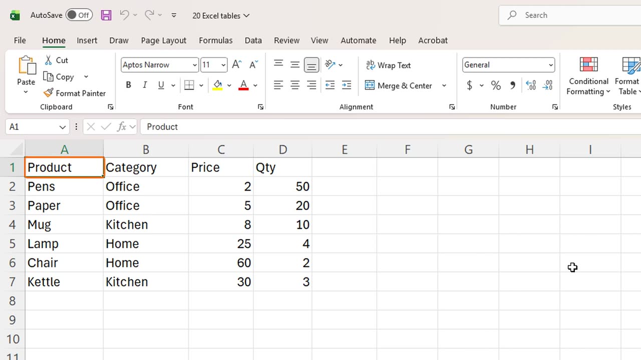
Here is a plain list of products, with a category, a price and a quantity. Click any cell inside it.
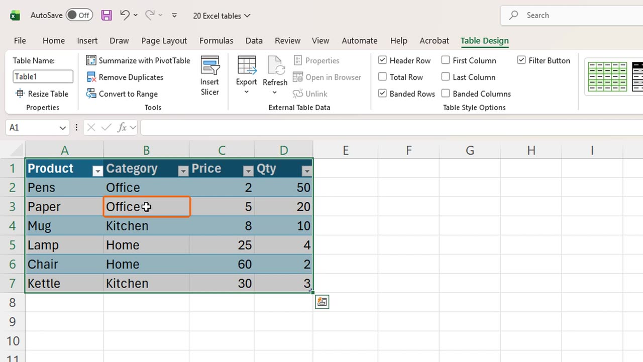
Press Control and T. Excel selects the whole list and asks if it has headers. It does, so press Enter.
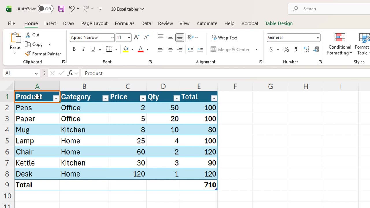
That is it. The rows now have alternating colors, which makes them easier to read, and every header has a filter arrow, just like in the last lesson.
A new tab also appears on the ribbon, called Table Design. Here you can pick another style, or give the Table a name.
Shortcut: Ctrl + T
3. Formulas that fill
Now let's add a column. Click E1, right next to the Table, type Total, and press Enter. The Table grows to include the new column.
In E2, type equals, then an opening square bracket, at sign, Price, closing bracket, times, and the same for Qty.
Press Enter. Excel fills the formula down the whole column by itself. No dragging, no copying.
The at sign means: this row. So the formula reads, the price in this row times the quantity in this row. Formulas like this are called structured references, and they are much easier to read than cell addresses.
=[@Price]*[@Qty]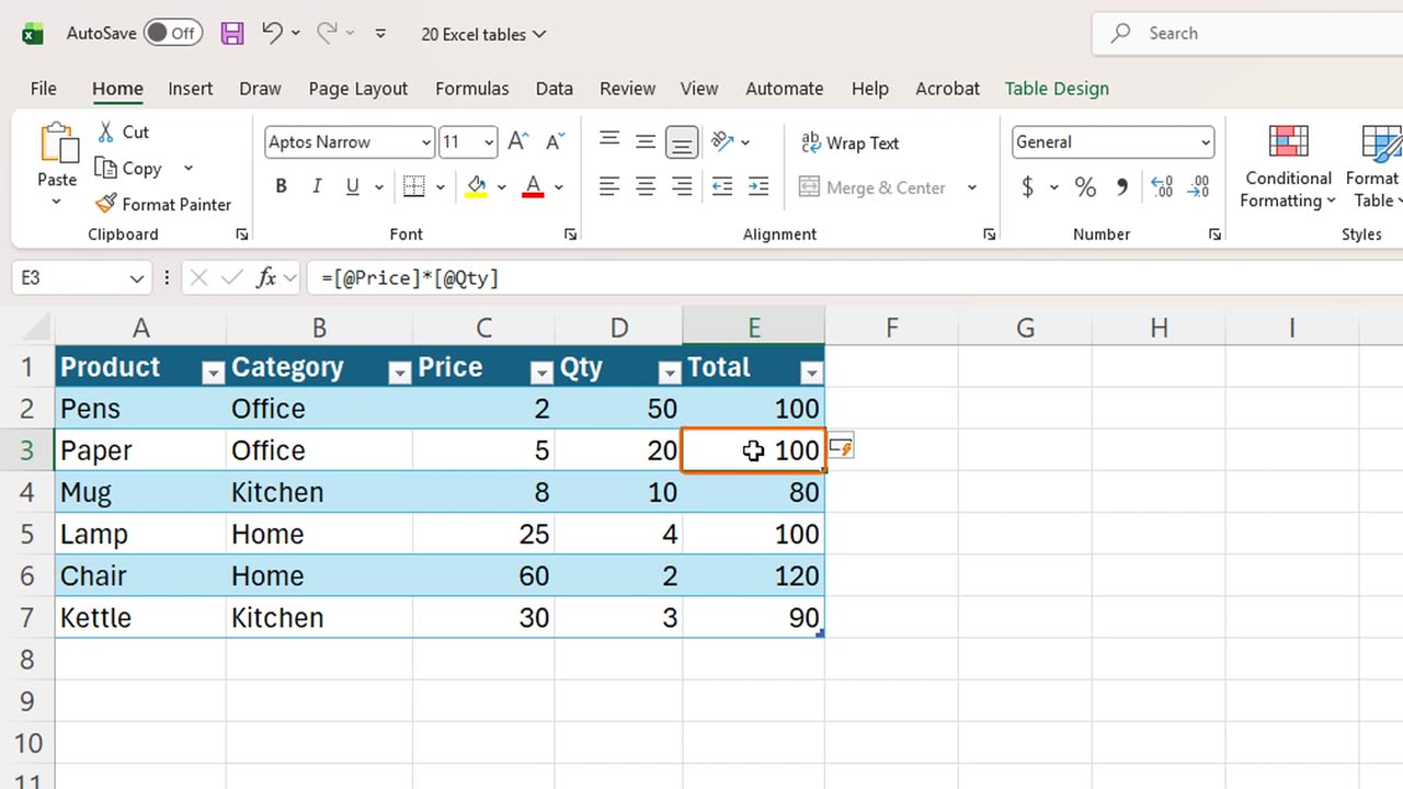
4. Rows that join
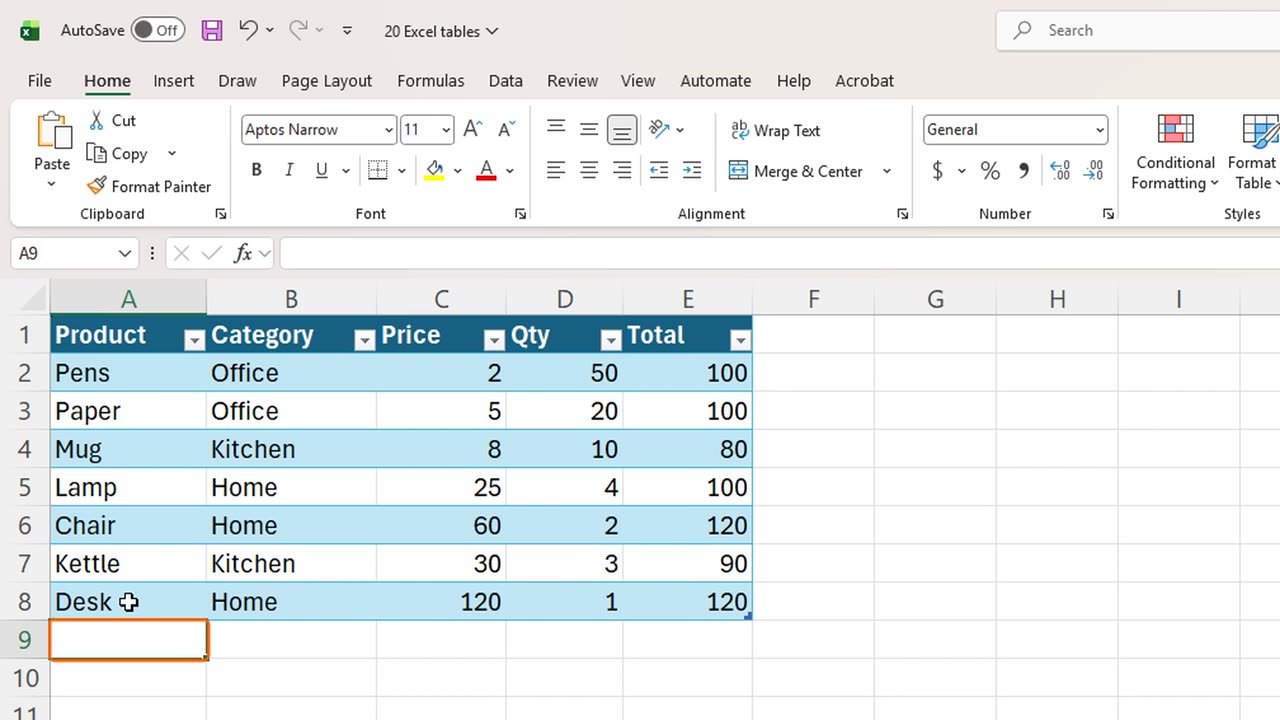
Now add a new product. Click A8, just under the Table, and type Desk, Home, one hundred and twenty, and one, pressing Tab between them.
The new row joined the Table. It got the same colors, and its Total was calculated automatically. Charts and formulas that use this Table will include it too.
5. Total Row
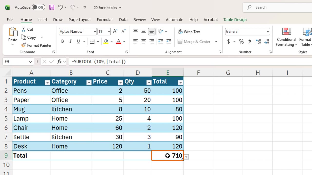
Finally, the Total Row. Click inside the Table and press Control, Shift and T. A row appears at the bottom, with the sum of the last column.
Click any cell in the Total Row, and an arrow lets you switch to an average, a count, a maximum, and more. If you filter the Table, the total only counts the visible rows.
6. Recap
Let's recap. Control T turns a list into a Table. New columns and rows join it automatically, formulas fill themselves, and Control Shift T adds a Total Row.
In the next lesson, you will learn how to find and remove duplicate entries safely.
If there is something you want to learn next, write it in the comments. Your requests decide what we teach in the next tutorials. Thanks for watching, and see you in the next one.
← Previous tutorial: Sort and Filter Data in Excel (Beginner Tutorial)
Next tutorial: Remove Duplicates in Excel (Find and Delete Repeats) →