Sort and Filter Data in Excel (Beginner Tutorial)
Sort A to Z, multi-level sort and filter by text, number and color.
- Intro
- Sort one column
- Sort by two columns
- Filter by text
- Filter by number
- Recap
Step by step
1. Intro
Welcome to Module 3, where we work with data. In this lesson, you will learn how to sort a list, and how to filter it, so you only see the rows you need.
Sorting changes the order of the rows. Filtering hides the rows you do not need, without deleting anything.
2. Sort one column
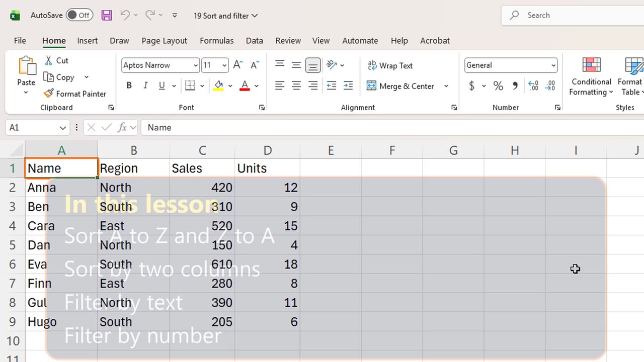
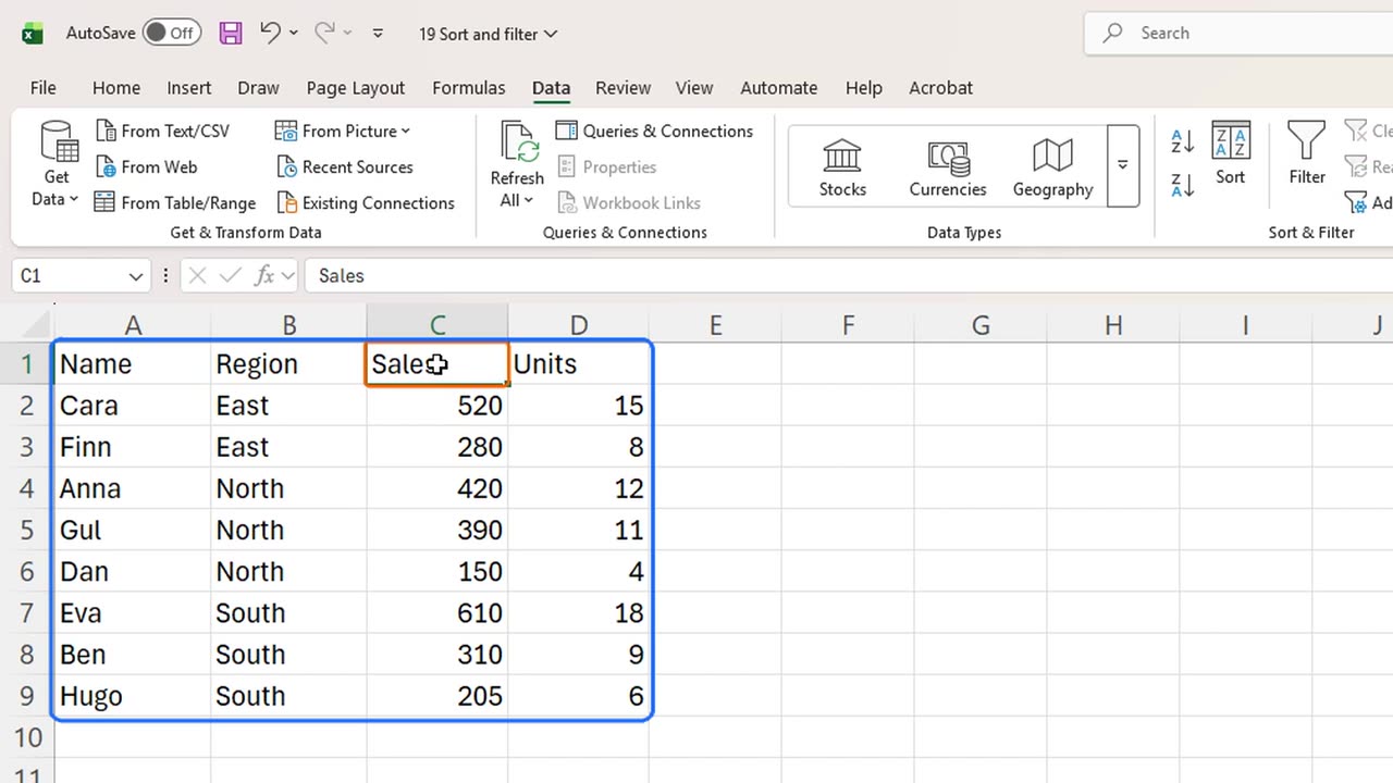
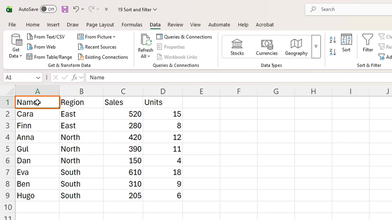
Here is a small sales list. Each row is one sales rep, with a region, sales and units sold.
Let's put the best sales at the top. Click any cell in the Sales column. On the Data tab, choose Sort Largest to Smallest. The shortcut is Alt, A, S, D.
Eva, with six hundred and ten, is now first. Notice that whole rows moved together: each name stayed with its own region and numbers.
This is why you click just one cell. If you select a single column and sort only that, the names and numbers get mixed up. Always let Excel sort the whole table.
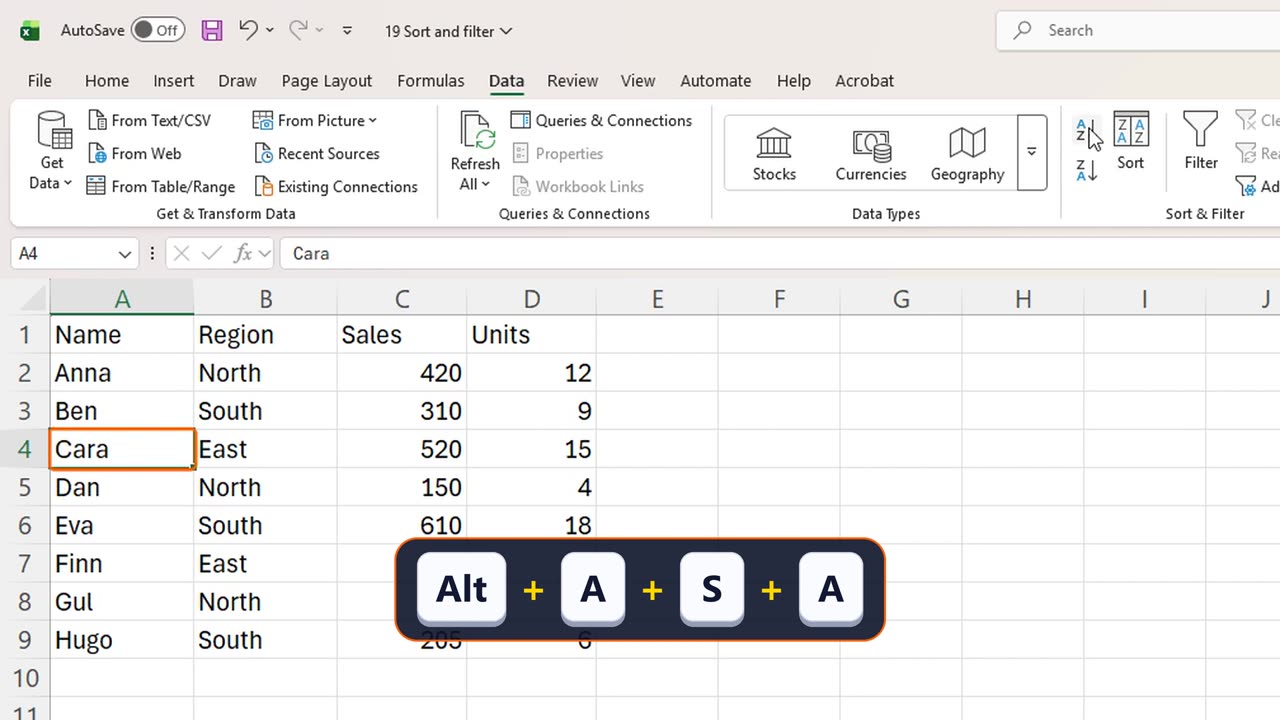
To sort by name, click a name and choose Sort A to Z, with Alt, A, S, A. The list is alphabetical again.
3. Sort by two columns
Now a sort on two levels. We want the regions in order, and inside each region, the biggest sales first. Open the Sort dialog with Alt, A, S, S.
In Sort by, choose Region, from A to Z. Then click Add Level. In Then by, choose Sales, and set the order to Largest to Smallest. Click OK.
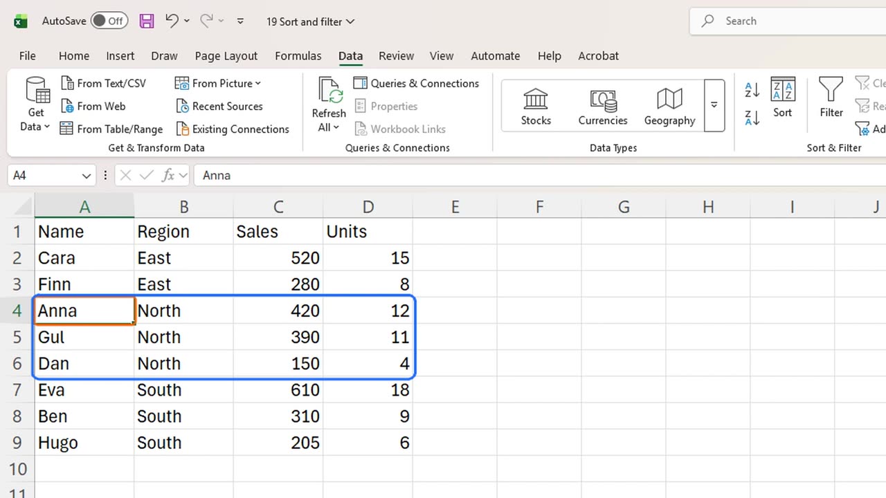
Look at the result. The regions are grouped: East, North, South. And inside North, Anna, Gul and Dan go from the highest sales to the lowest.
4. Filter by text
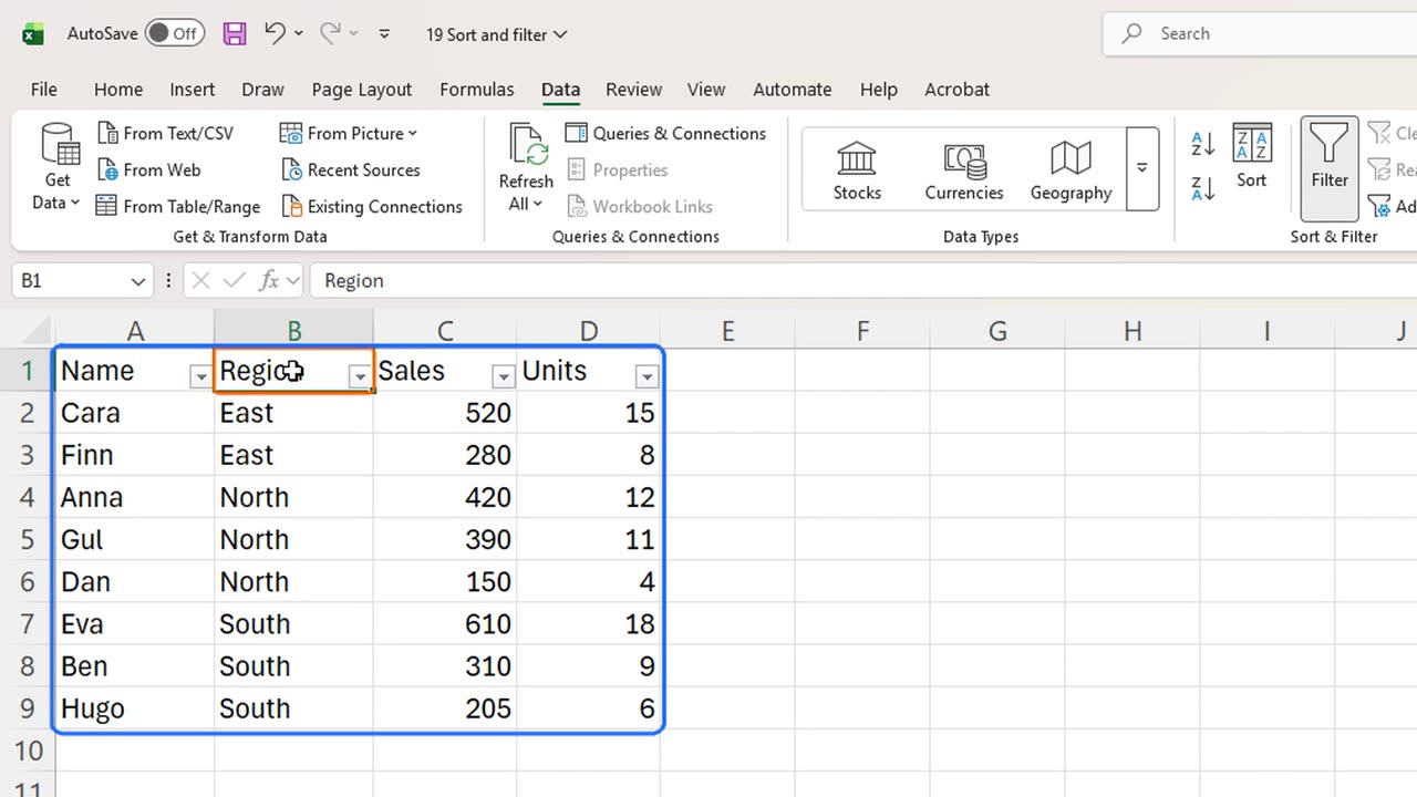
Next, filtering. Press Control, Shift and L. Small arrows appear on every header. This works the same in every language version of Excel.
Let's show only the North region. Click the arrow on the Region header, or press Alt and the down arrow. Type North in the search box, and press Enter.
Only three rows are left. The other rows are hidden, not deleted. The blue row numbers and the funnel on the arrow tell you a filter is on.
To remove it, open the same arrow and choose Clear Filter From Region. All eight rows are back.
5. Filter by number
Numbers have their own filters. Open the Sales arrow, choose Number Filters, then Greater Than. Type three hundred, and press Enter.
Now we only see the reps who sold more than three hundred. The status bar at the bottom tells you how many records were found.
The same menu can also filter by cell color or font color, which is handy when someone has highlighted rows by hand.
When you are done, press Control, Shift, L again. The arrows disappear, and every filter is removed at once.
6. Recap
Let's recap. Sort with one cell selected, so whole rows move together. Use the Sort dialog for two levels. Control Shift L turns filters on and off, and filters only hide rows.
In the next lesson, you will turn this list into an Excel Table, which gives you filters, colors and growing formulas automatically.
If there is something you want to learn next, write it in the comments. Your requests decide what we teach in the next tutorials. Thanks for watching, and see you in the next one.
← Previous tutorial: Excel Formula Auditing: Trace Precedents and Show Formulas
Next tutorial: Excel Tables: Why You Should Use Them (Ctrl + T) →