One Excel Chart, Any Region: Drop-Down + FILTER
A drop-down list drives FILTER, and FILTER drives one chart; plus the empty-choice error and its one-argument fix.
- One chart, any region
- The drop-down
- FILTER the row
- The chart
- The empty trap
Step by step
1. One chart, any region
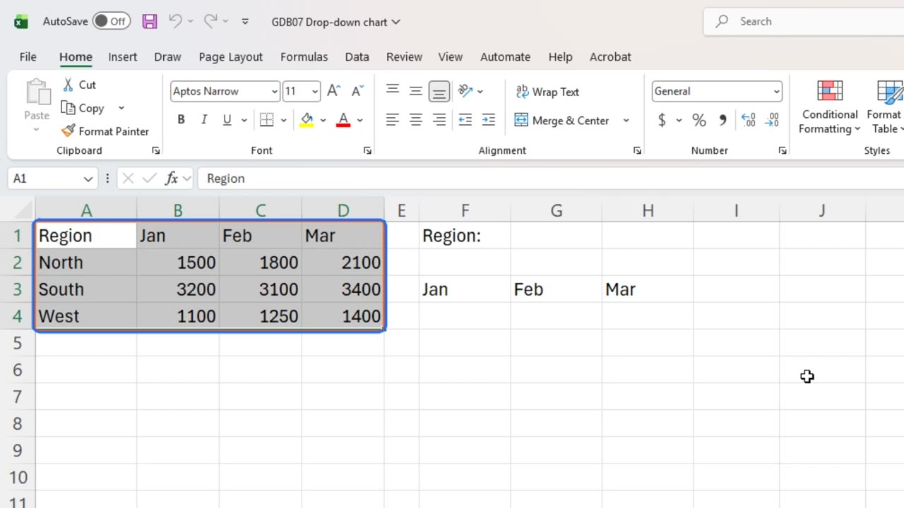
Three regions do not need three charts. One chart and a drop-down can show any of them, and the dashboard stays clean.
2. The drop-down
Start with the drop-down. Click G1, then on the Data tab, click Data Validation.
In the Allow box, choose List.
Click the Source box and type the region cells: equals A2 colon A4. Then click OK.
You can also open this window from the keyboard: Alt, A, V, V.
Now pick a region. Type North in G1.
=$A$2:$A$4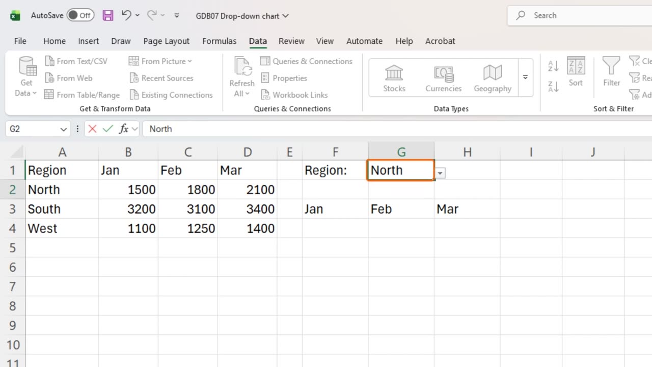
3. FILTER the row
Next, pull that region's numbers. In F4, type equals FILTER, the monthly figures, then the Region column equals G1.
One formula spills the three months for North across the row.
=FILTER(B2:D4,A2:A4=G1)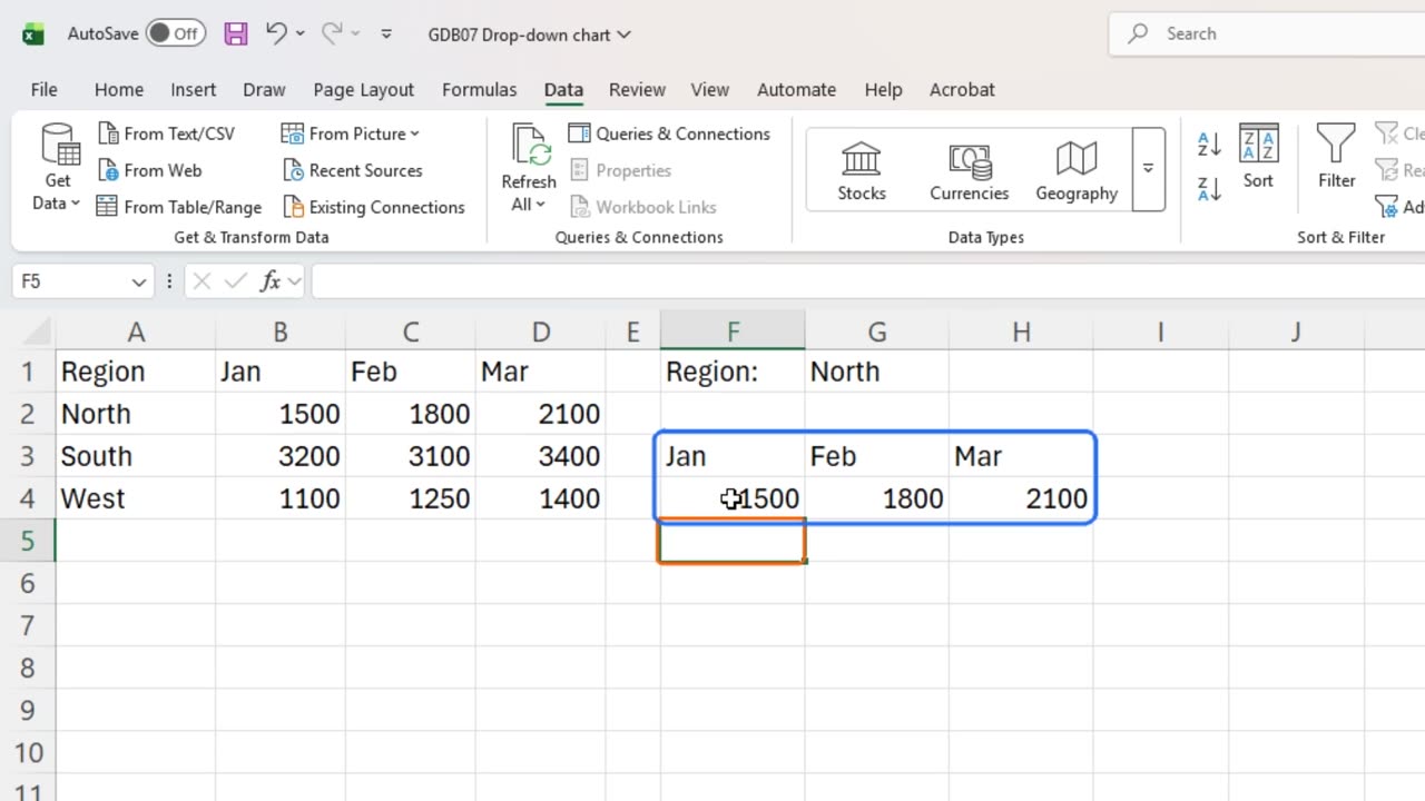
4. The chart
Select the headings and that row, F3 to H4. On the Insert tab, click the column chart button and pick the first chart.
Or press Alt and F1 for the same chart in one step.
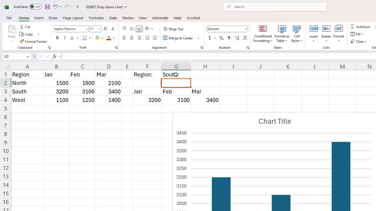
Now change the region. Click G1 and type South.
The numbers change, and the chart redraws by itself. One chart, every region.
5. The empty trap
Here is the trap. Someone clears the drop-down. Click G1 and press Delete.
FILTER finds no matching row and shows a calc error, and the chart goes blank.
FILTER has a third argument for exactly this. Click F4, and retype the formula with comma, quote, Pick a region, quote, at the end.
Now an empty choice shows a friendly message instead of an error. Type North again, and everything comes back.
Would you control your charts with a drop-down, or with slicers? Tell me in the comments.
=FILTER(B2:D4,A2:A4=G1,"Pick a region")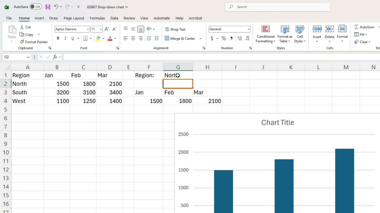
← Previous tutorial: Green and Red KPI Arrows in Excel Without a Formula
Next tutorial: Excel Icon Sets: Why Zero Gets a Green Arrow →