Excel Icon Sets: Why Zero Gets a Green Arrow
Add variance arrows from the keyboard, then see the percent-threshold trap that turns a zero green, and where to fix it.
- Ahead or behind
- The variance
- Icon sets
- The percent trap
Step by step
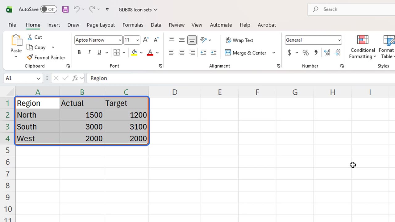
1. Ahead or behind
Are we ahead of target or behind? A dashboard should answer that with one glance, not with subtraction in your head.
2. The variance
First, the variance. In D1, type Variance. In D2, type equals B2 minus C2, actual minus target.
Fill it down to row four: North is three hundred ahead, South one hundred behind, and West exactly on target.
=B2-C2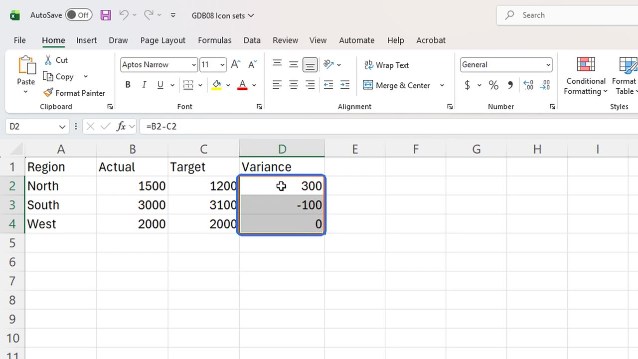
3. Icon sets
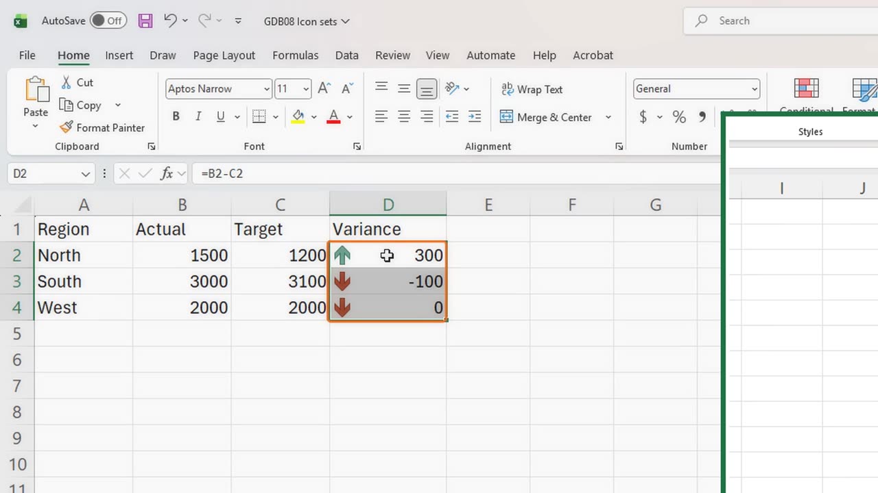
Now the icons. Select the variances and press Alt, H, L, I. That is Conditional Formatting, Icon Sets.
Press Enter to take the first set: three coloured arrows.
4. The percent trap
Green up for North, red down for South. But look at West: exactly on target, a variance of zero, and it got a red arrow too.
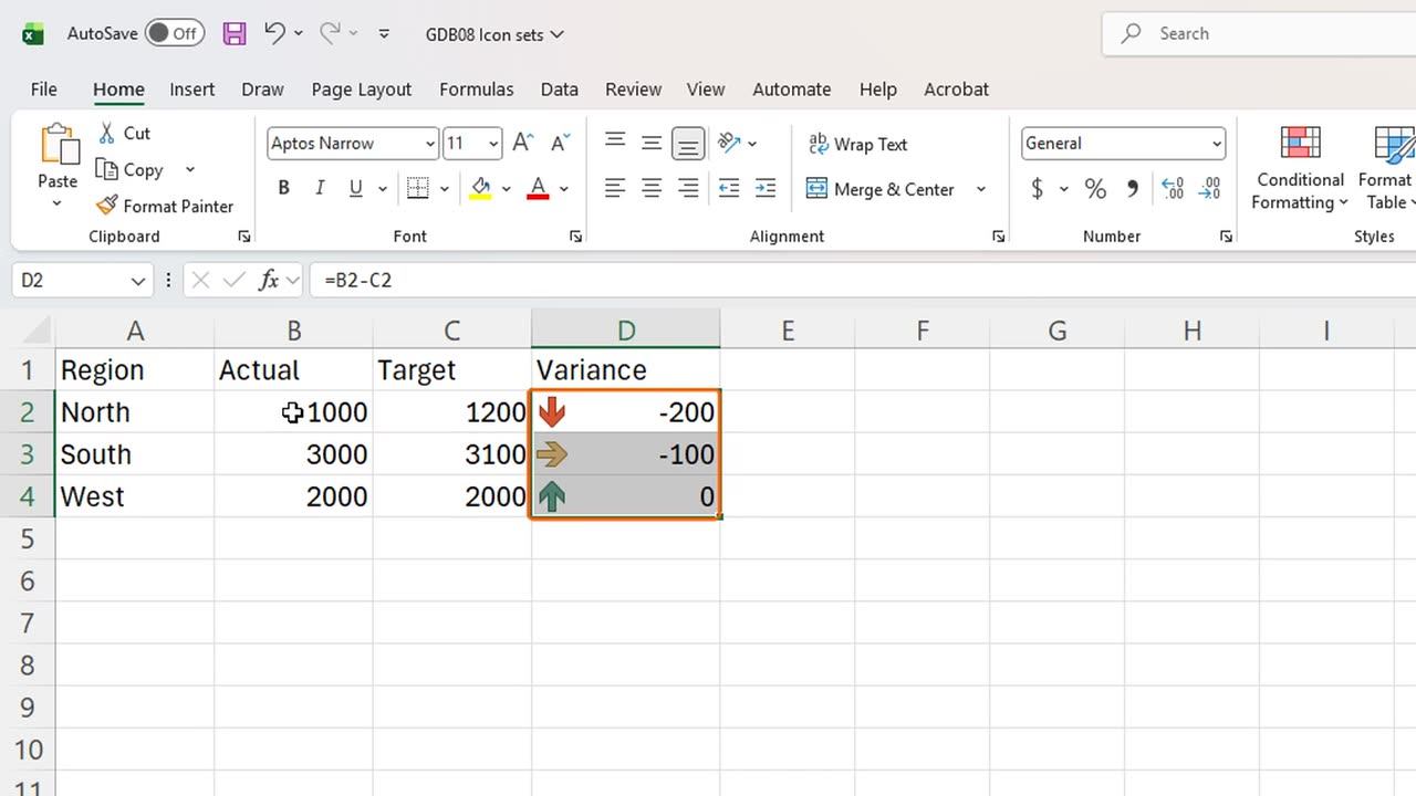
That is the trap, and it gets stranger. Give North a bad month: type one thousand as its actual.
West did not change at all, still zero, but now its arrow is green, as if it were the star of the team.
Icon sets compare each value with the others, in percent of the range, not with zero. Zero was the worst third before, and now it is the best third.
The fix lives in Manage Rules: press Alt, H, L, R.
Edit the icon set rule and change its type from Percent to Number, with green from zero and above. Then the arrows follow the target, not each other.
Arrows, traffic lights or flags: which icons do you use in your reports? Tell me in the comments.
← Previous tutorial: One Excel Chart, Any Region: Drop-Down + FILTER
Next tutorial: Excel's Live Picture Trick for Dashboards →