Green and Red KPI Arrows in Excel Without a Formula
One custom number format turns changes into coloured up and down arrows; plus the bright-green mistake and its fix.
- Arrows without formulas
- The change
- A custom format
- The lime trap
- Live
Step by step
1. Arrows without formulas
Plus fourteen point five percent, minus three point eight. A KPI card should not make you read signs. It should show you, in colour, with an arrow.
2. The change
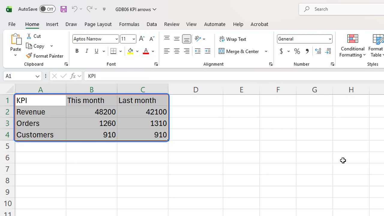
First, the change. In D1 type Change, and in D2 type equals B2 divided by C2, minus one.
Fill it down to row four. Raw decimals, hard to read.
=B2/C2-1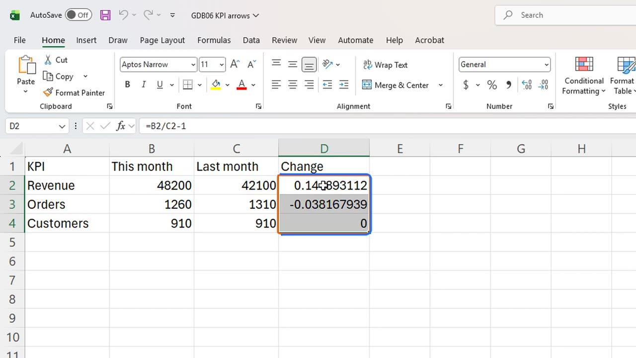
3. A custom format
Select the three results and press Control and 1. Format Cells opens on the Number tab.
Press Alt and C for the category list, End to jump to Custom, and Alt and T for the Type box.
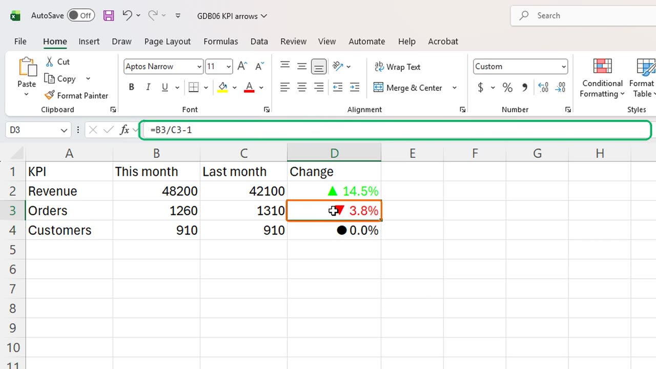
Type the code. Three parts, separated by semicolons: positive, negative, zero. Green with an up arrow, red with a down arrow, and a dot for no change.
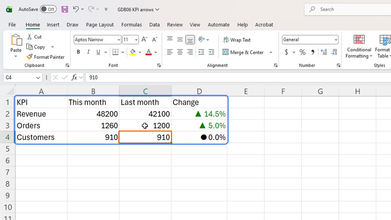
Arrows and colours, and the cells still hold plain numbers. The minus sign is gone, because the arrow already says down.
4. The lime trap
But here is the trap. Look at that green. Excel's Green is a bright lime, and on a white card it is almost unreadable.
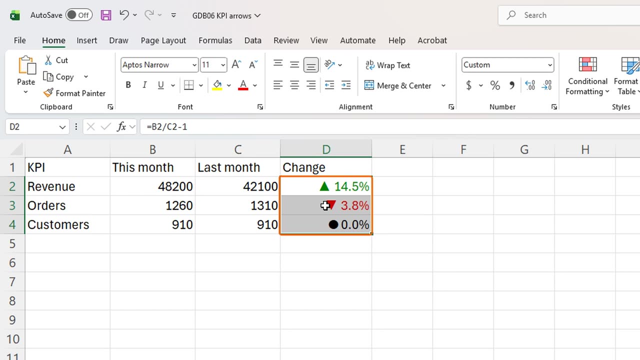
Open the same box again, and replace Green with Color ten. That is Excel's dark green from its colour palette.
Now it reads like a real dashboard: a calm green for good news, red for bad.
5. Live
And it is live. Last month's orders were really twelve hundred. Type that in C3.
Orders flip to a green up arrow, plus five percent. No formula changed, only the number.
Which KPI would you put on a card like this? Write it in the comments.
← Previous tutorial: Tiny Charts Inside Excel Cells (Sparklines)
Next tutorial: One Excel Chart, Any Region: Drop-Down + FILTER →