Tiny Charts Inside Excel Cells (Sparklines)
Add sparklines from the keyboard, watch them update live, and avoid the scale trap that makes small numbers look big.
- Trends at a glance
- Insert sparklines
- Live updates
- The scale trap
Step by step
1. Trends at a glance
A row of six numbers hides its story. Is this rep growing or slipping? A tiny chart inside the cell answers before you finish reading.
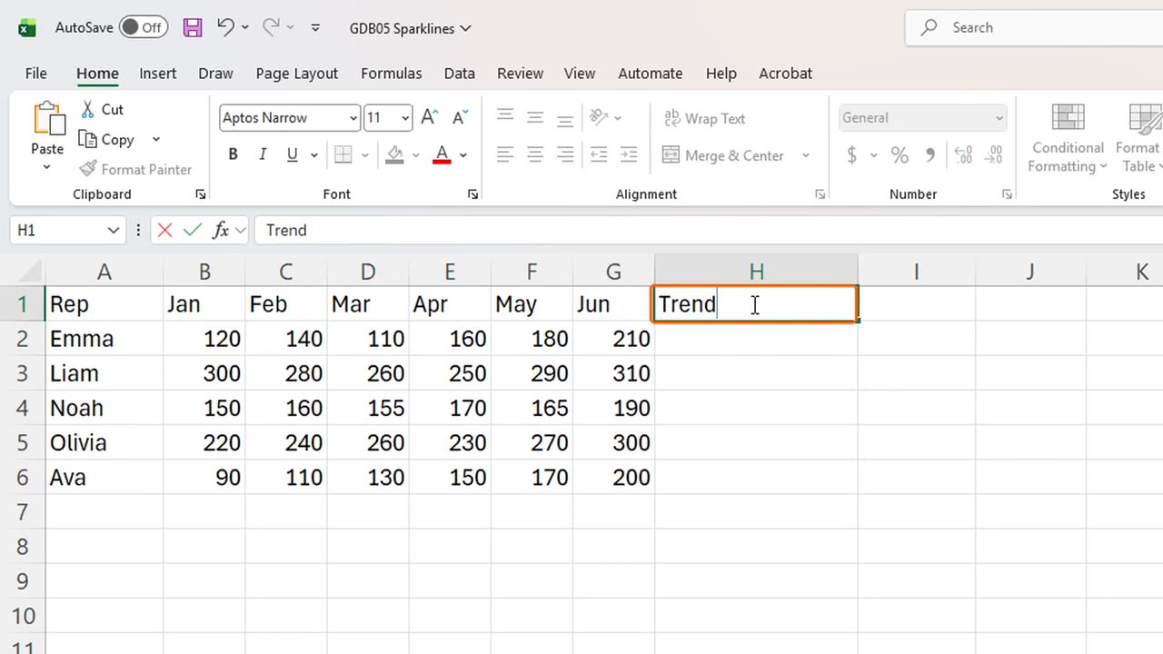
These are sparklines. First, a place for them: in H1, type Trend.
2. Insert sparklines
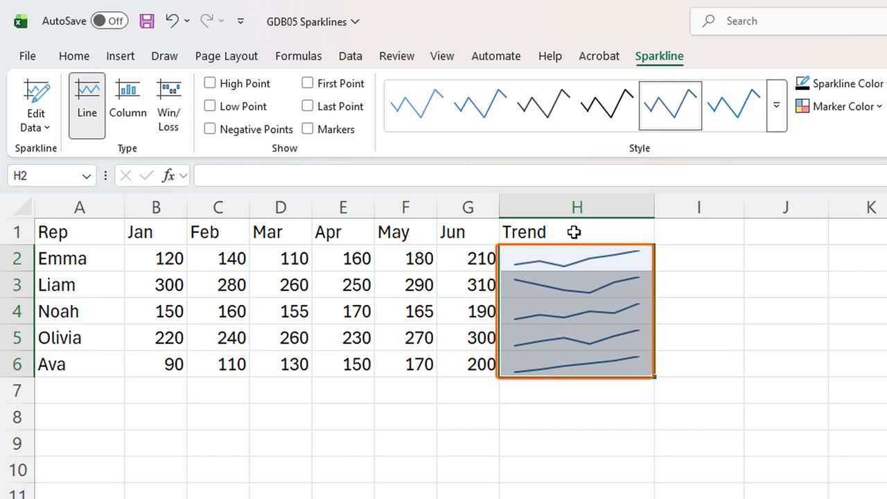
Select the empty cells H2 to H6, where the little charts will live.
Press Alt, N, S, L. That is Insert, Sparklines, Line.
Excel already knows where the sparklines go. It only asks for the data. Type B2 colon G6, and press Enter.
Five rows, five tiny line charts. Emma climbs steadily, Liam dips in spring and recovers, and Ava rises every single month.
Sparklines sit inside the cells, so they move, sort and resize with the grid. No floating chart to drag around.
3. Live updates
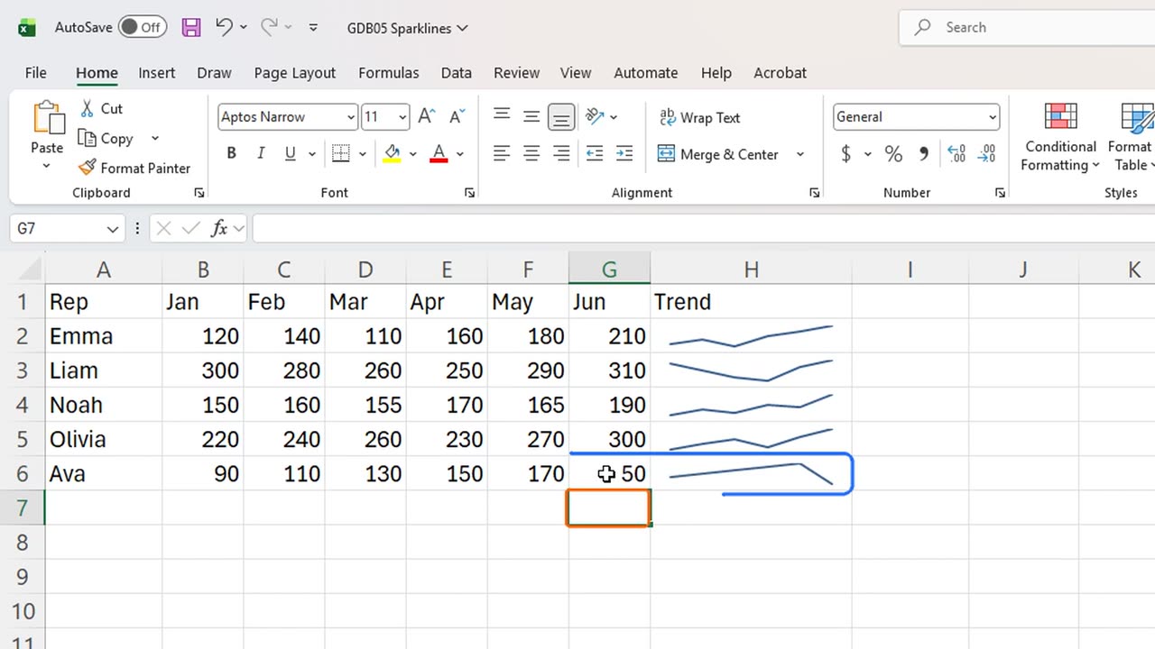
They are live too. Type fifty in Ava's June, and watch her line drop at the end.
4. The scale trap
Now the trap. Add a total in column I: in I1 type Total, and in I2 sum B2 to G2, then fill down.
Emma's line looks just as tall as Liam's, yet Liam sold almost twice as much. Each sparkline stretches to fill its own cell.
So read a sparkline for its shape, growing or falling, and read the total for its size. Together they tell the full story.
Would you add sparklines to your own reports, or do you prefer full charts? Tell me in the comments.
=SUM(B2:G2)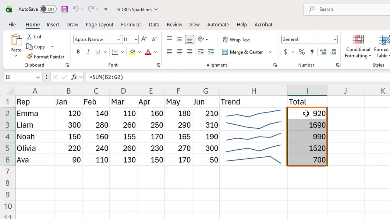
← Previous tutorial: An Excel Chart Title That Updates Itself
Next tutorial: Green and Red KPI Arrows in Excel Without a Formula →