Which Chart Should You Use? (Excel Chart Types Guide)
Pick the best chart for comparison, trend, share and relationship.
- One question
- Compare
- Trend
- Share
- Relationship
- The fake trend
- Recap
Step by step
1. One question
The wrong chart hides your point, the right one makes it obvious. Ask one question first: what am I showing?
Four answers: a comparison, a trend, a share of a whole, or a relationship. Each one has its chart.
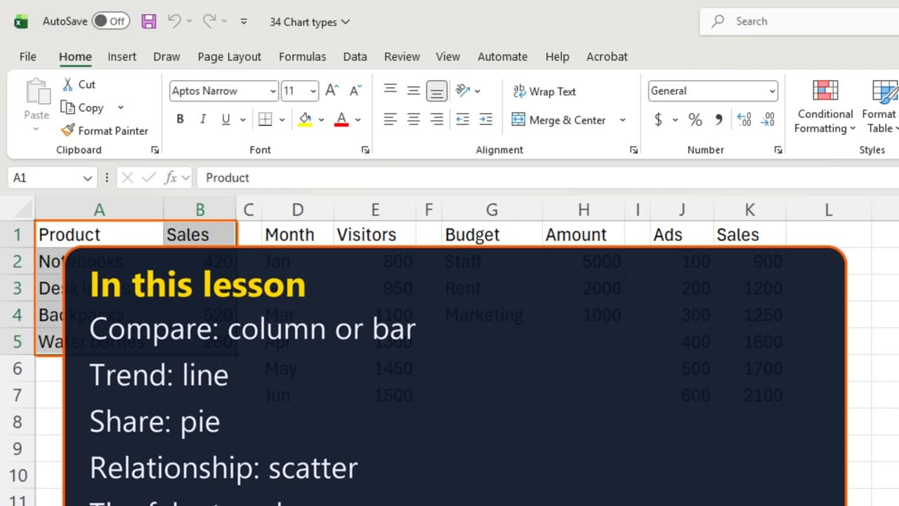
2. Compare
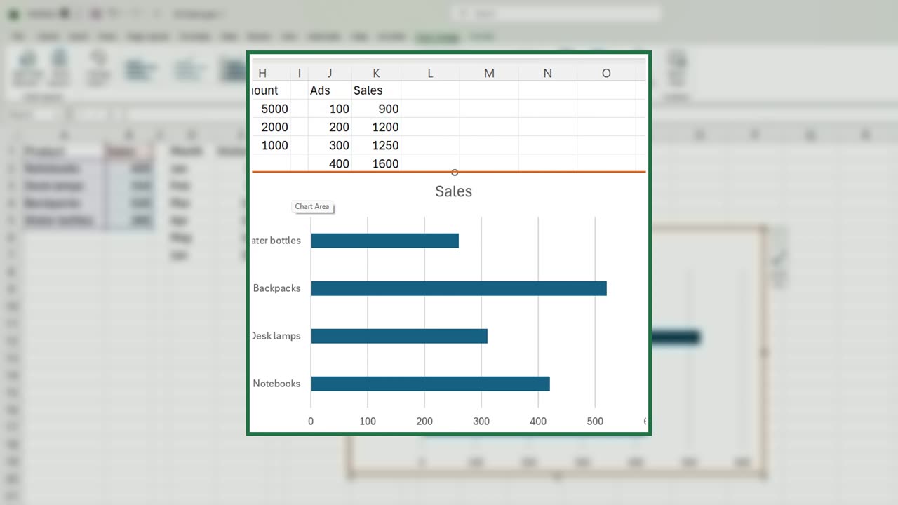
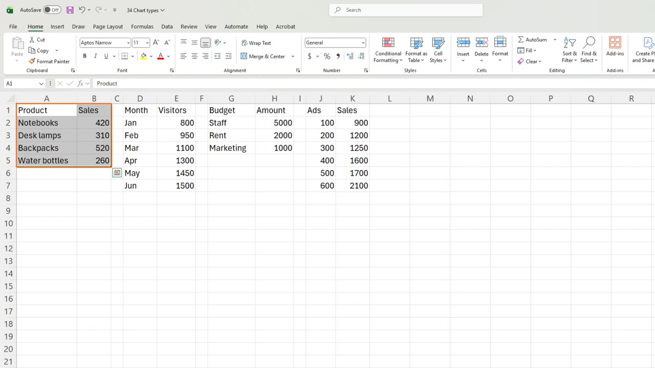
Comparison first: sales by product. Select A1 to B5 and press Alt and F1. Columns let the eye compare heights.
With long product names, switch to Bar. Horizontal bars leave room for the labels.
3. Trend
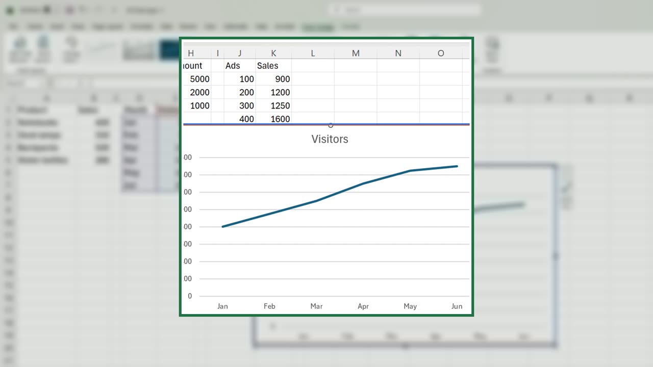
Press Delete to remove it. Next, a trend: monthly visitors. Select D1 to E7, Alt and F1, and switch to Line.
A line connects the months, so your eye follows the direction: up all spring.
Quick pause: if this saves you some guessing, a like really helps the channel. Two charts to go, and then the trap.
4. Share
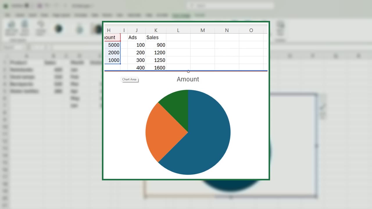
Delete it. A share of one whole: the budget split. Select G1 to H4, Alt and F1, and switch to Pie. Three slices, easy to read.
5. Relationship
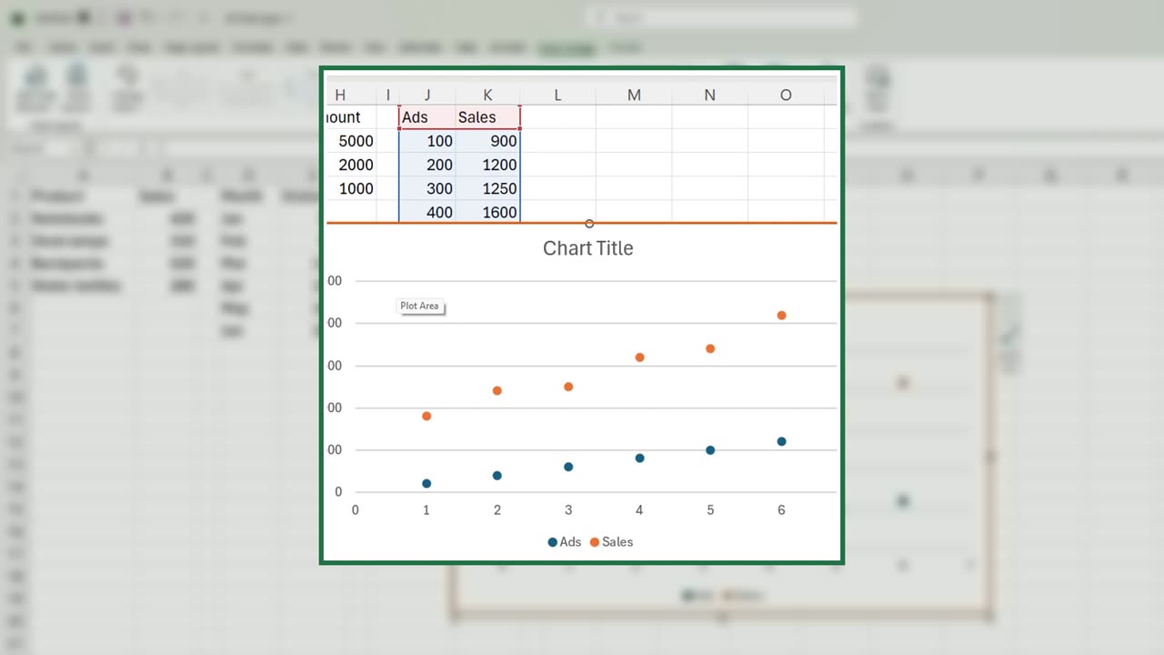
Delete it. A relationship: does more advertising bring more sales? Select J1 to K7, Alt and F1, and switch to Scatter.
Each dot is one week. The dots climb from left to right, so yes: more ads, more sales.
6. The fake trend
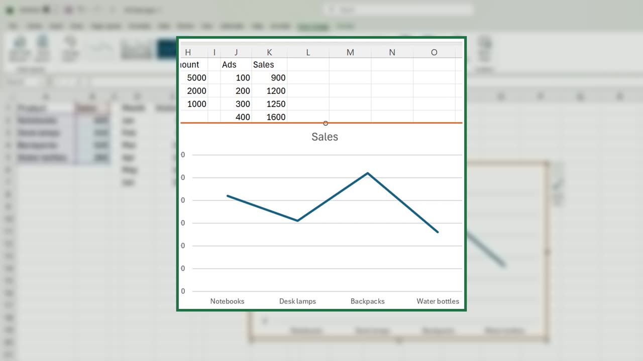
Now the trap. Select the products again, Alt and F1, and switch to Line. The line rises and falls as if products had a trend over time.
But products are not a timeline. That line means nothing. Use lines only when the categories follow each other in time.
7. Recap
Recap: compare with columns or bars, trends with lines, one whole with a pie, relationships with a scatter.
In the next lesson, you will learn the twenty-five keyboard shortcuts that save the most time.
Which chart do you see misused most often at work? Tell me in the comments.
← Previous tutorial: Build a Simple Excel Dashboard (Beginner Friendly)
Next tutorial: 25 Excel Keyboard Shortcuts Every Beginner Should Know →