Excel Slicers: Filter PivotTables with Buttons
Add slicers and timelines to filter with a click.
- Buttons, not lists
- The PivotTable
- Add a slicer
- One click
- A timeline
- What slicers miss
- Recap
Step by step
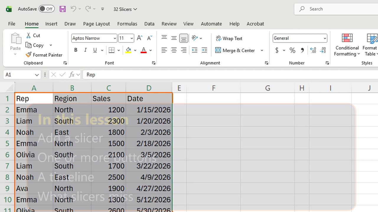
1. Buttons, not lists
Filtering a PivotTable with drop-down lists is slow. A slicer gives you buttons: one click, and the report shows one region.
You will add a slicer, pick one or two regions, filter by month with a timeline, and see what a slicer cannot reach.
2. The PivotTable
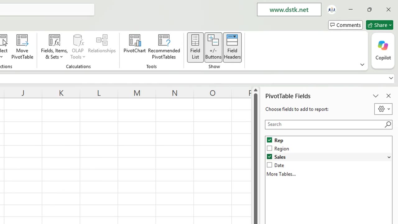
First a PivotTable at F1: Control and T, Enter, Alt, N, V, T, then tick Rep and Sales.
Shortcut: Ctrl + T
3. Add a slicer
With a cell inside the PivotTable selected, insert a slicer: Alt, N, S, F.
Press Down to reach Region, Space to tick it, and Enter.
4. One click
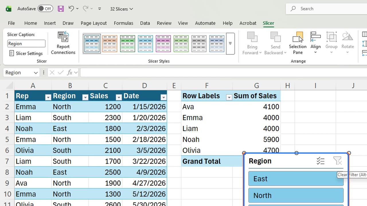
One button per region. Click North. Only Ava and Emma are left: eight thousand one hundred.
Hold Control and click South to add it. The buttons you picked stay colored, the others turn grey.
To see everything again, click the clear filter icon in the slicer's corner.
Quick pause: if your reports just got clickable, a like really helps the channel. Next, months.
5. A timeline
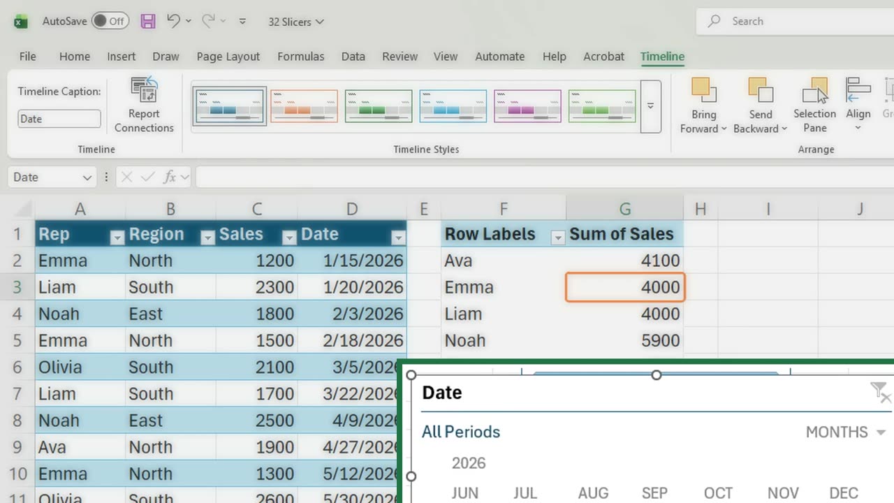
For dates there is a special slicer, the timeline. Click in the PivotTable and press Alt, N, S, T, then Space and Enter.
Click June. The report shows June only: Ava and Noah, three thousand eight hundred.
6. What slicers miss
Now the trap. Next to the report, in I1, type equals SUM of C2 to C13.
Twenty two thousand seven hundred, the whole year. Slicers and timelines filter only the PivotTable. Formulas on the source data never see them.
So any number that should follow the buttons must come from the PivotTable itself.
=SUM(C2:C13)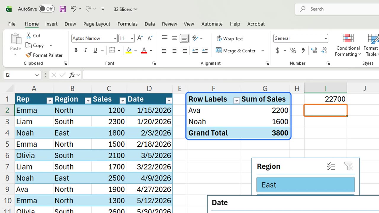
7. Recap
Recap: Alt, N, S, F adds a slicer, Control-click picks more than one, Alt, N, S, T adds a timeline, and only the PivotTable follows them.
In the next lesson, you will put PivotTables, charts and slicers together into a simple dashboard.
Which field would you put on a slicer in your own reports? Tell me in the comments.
← Previous tutorial: PivotTable Grouping and Calculated Fields
Next tutorial: Build a Simple Excel Dashboard (Beginner Friendly) →