Remove Duplicates in Excel (Find and Delete Repeats)
Highlight and remove duplicate values safely.
- Intro
- Highlight first
- Remove Duplicates
- What counts as a duplicate
- UNIQUE: a safe copy
- Recap
Step by step
1. Intro
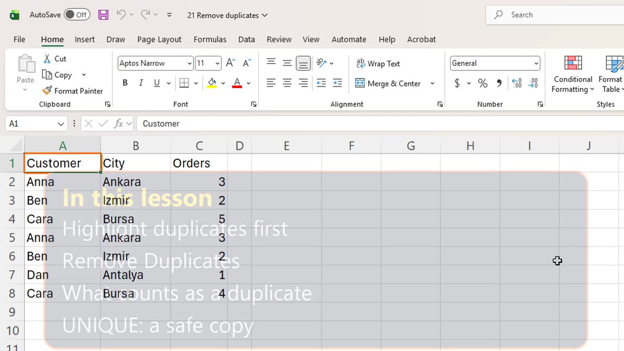
Welcome back. Lists copied from different places often contain the same entry twice. In this lesson, you will learn to find duplicates, and remove them safely.
The safe order is simple: first look at the duplicates, then remove them, and keep the original data until you are sure.
2. Highlight first
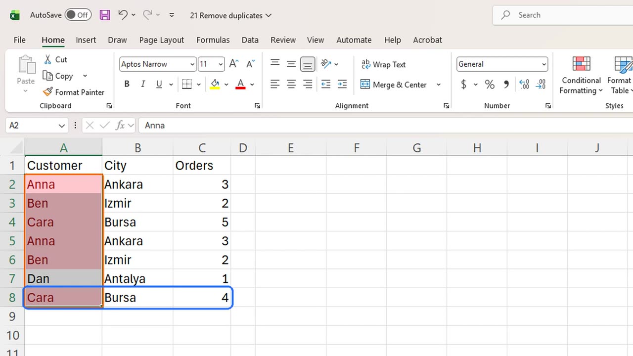
Here is a customer list with seven rows. Some customers appear more than once.
Select the names, from A2 to A8. On the Home tab, open Conditional Formatting, Highlight Cells Rules, Duplicate Values. Press Enter to accept the red color. The keys for this are Alt, H, L, H, D.
Anna, Ben and Cara are now red. Nothing was deleted, so this step is always safe. It shows you what you are about to remove.
Look closely at Cara. One row has five orders, the other has four. Are these really the same entry? Keep that question in mind.
3. Remove Duplicates
Now remove them. Click any cell in the list, and on the Data tab choose Remove Duplicates, with Alt, A, M.
Excel selects the whole list and shows its columns. All three are checked. That means a row counts as a duplicate only if the customer, the city and the orders are all the same.
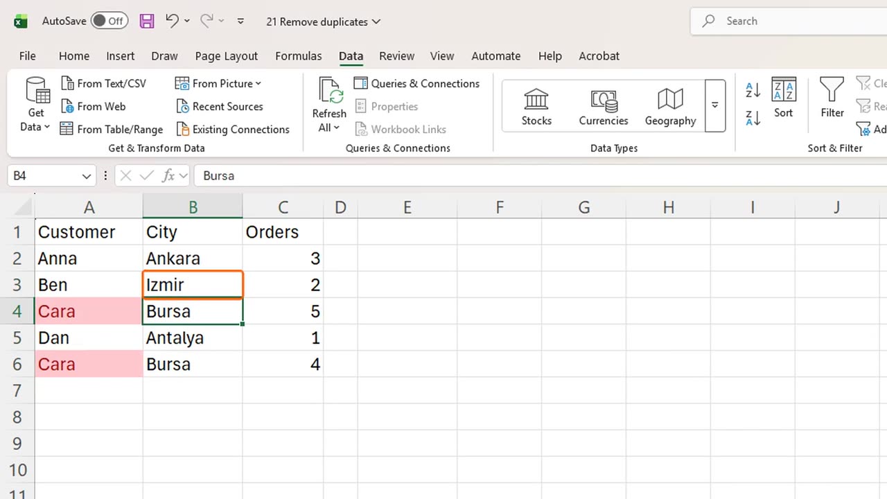
Click OK. Excel says two duplicate values were removed, and five unique values remain. Press Enter to close the message.
4. What counts as a duplicate
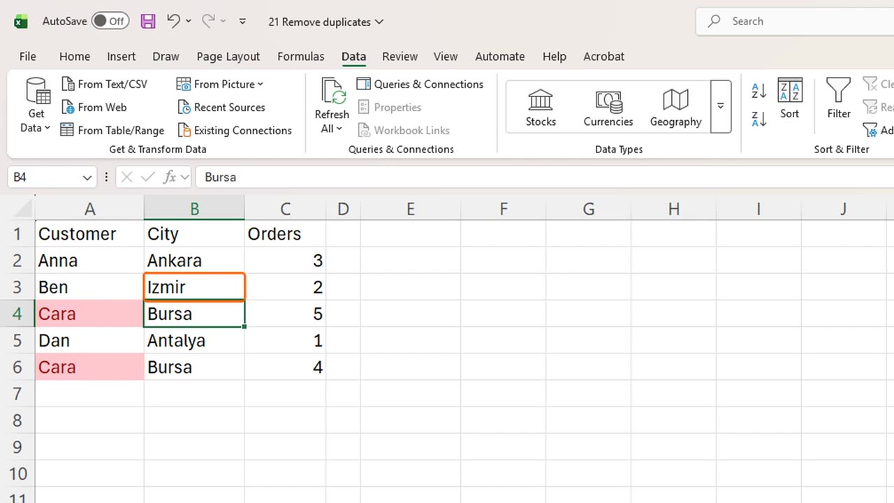
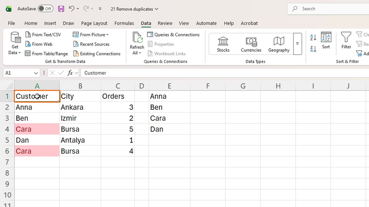
The second Anna and the second Ben are gone. But both Cara rows stayed, because their orders are different. Excel only removes rows that match in every checked column.
If you wanted one row per customer, you would uncheck the other columns and leave only Customer. Decide this carefully, because Remove Duplicates deletes rows. If you make a mistake, Control Z brings them back.
5. UNIQUE: a safe copy
There is also a way that never deletes anything: the UNIQUE function. Click E1, and type equals UNIQUE, open bracket, A2 to A6, close bracket.
Press Enter. You get each name once, in a separate list, and the original data is untouched. If the list changes, this result updates by itself.
=UNIQUE(A2:A6)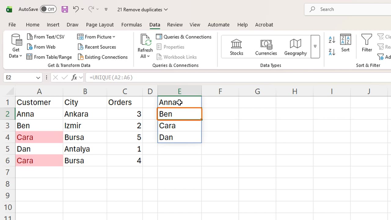
6. Recap
Let's recap. Highlight duplicates first, so you see them. Remove Duplicates deletes rows that match in every checked column. And UNIQUE gives you a clean list without touching the original.
In the next lesson, you will create drop-down lists, so people can only type allowed values.
If there is something you want to learn next, write it in the comments. Your requests decide what we teach in the next tutorials. Thanks for watching, and see you in the next one.
← Previous tutorial: Excel Tables: Why You Should Use Them (Ctrl + T)
Next tutorial: Excel Data Validation: Drop-Down Lists and Rules →