Excel Named Ranges (Make Formulas Easy to Read)
Give ranges names with the Name Box and use them in formulas.
- Intro
- Naming a range
- Names in formulas
- Jump to a name
- Easy changes
- Naming rules
- Recap
Step by step
1. Intro
Welcome back. In this lesson, you will learn to give names to cells and ranges, so that your formulas read like sentences instead of codes.
Compare these two formulas. Equals SUM of B2 to B6, and equals SUM of Sales. The second one tells you exactly what it adds up, and you do not need to remember any addresses.
2. Naming a range
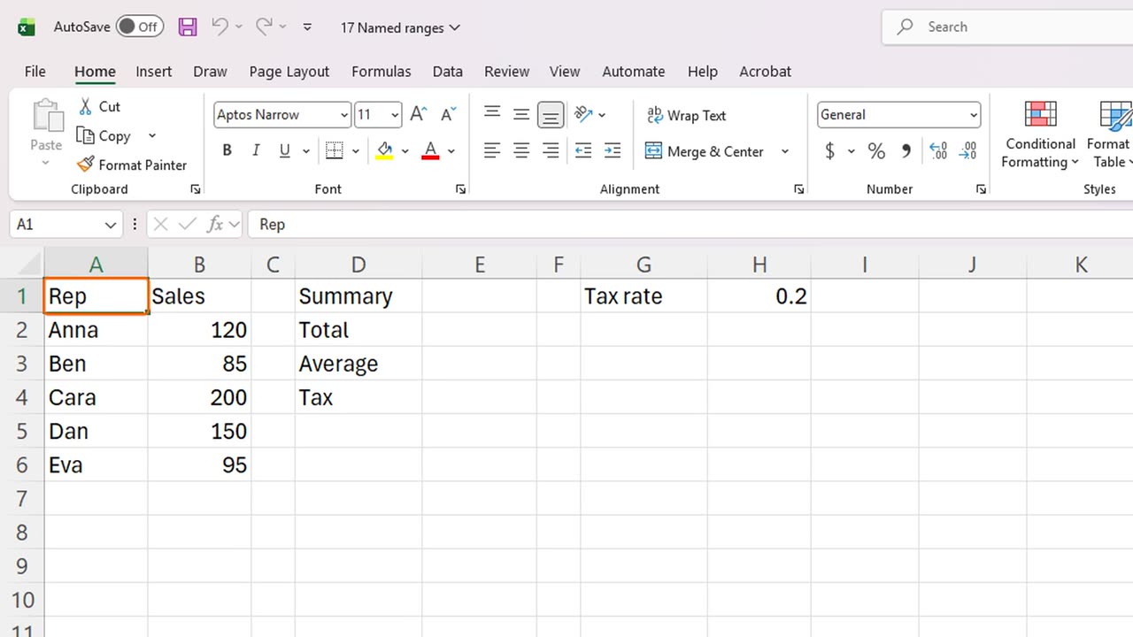
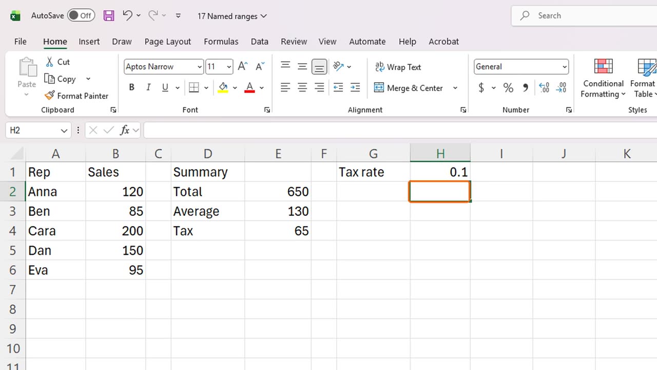
Here are five sales figures, and a tax rate in cell H1. We will name the sales, and the tax rate.
Select the five sales numbers, B2 to B6. Then click the Name Box, at the left of the formula bar. It currently shows the address of the selected cell.
Type the name Sales, and press Enter. The range now has a name.
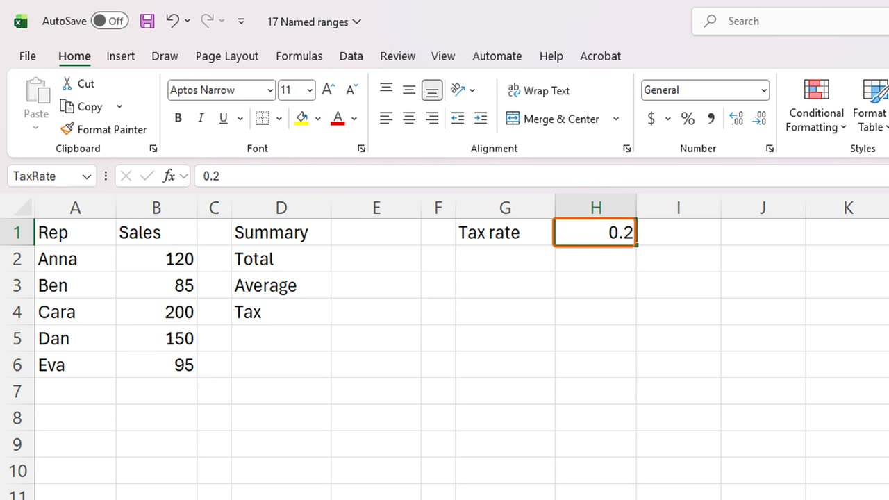
Now the tax rate. Click H1, click the Name Box, type TaxRate as one word, and press Enter.
3. Names in formulas
Now let's use the names. Click E2 and type equals SUM, open bracket, Sales, close bracket. Notice that Excel suggests your name while you type.
The total is six hundred and fifty. In E3, type equals AVERAGE of Sales.
And in E4, the tax: equals SUM of Sales, star, TaxRate. Read it aloud: the sum of sales times the tax rate. It reads like a sentence.
A name is always absolute, as if it had dollar signs. So you can copy a formula anywhere, and the name never drifts.
=SUM(Sales)=AVERAGE(Sales)=SUM(Sales)*TaxRate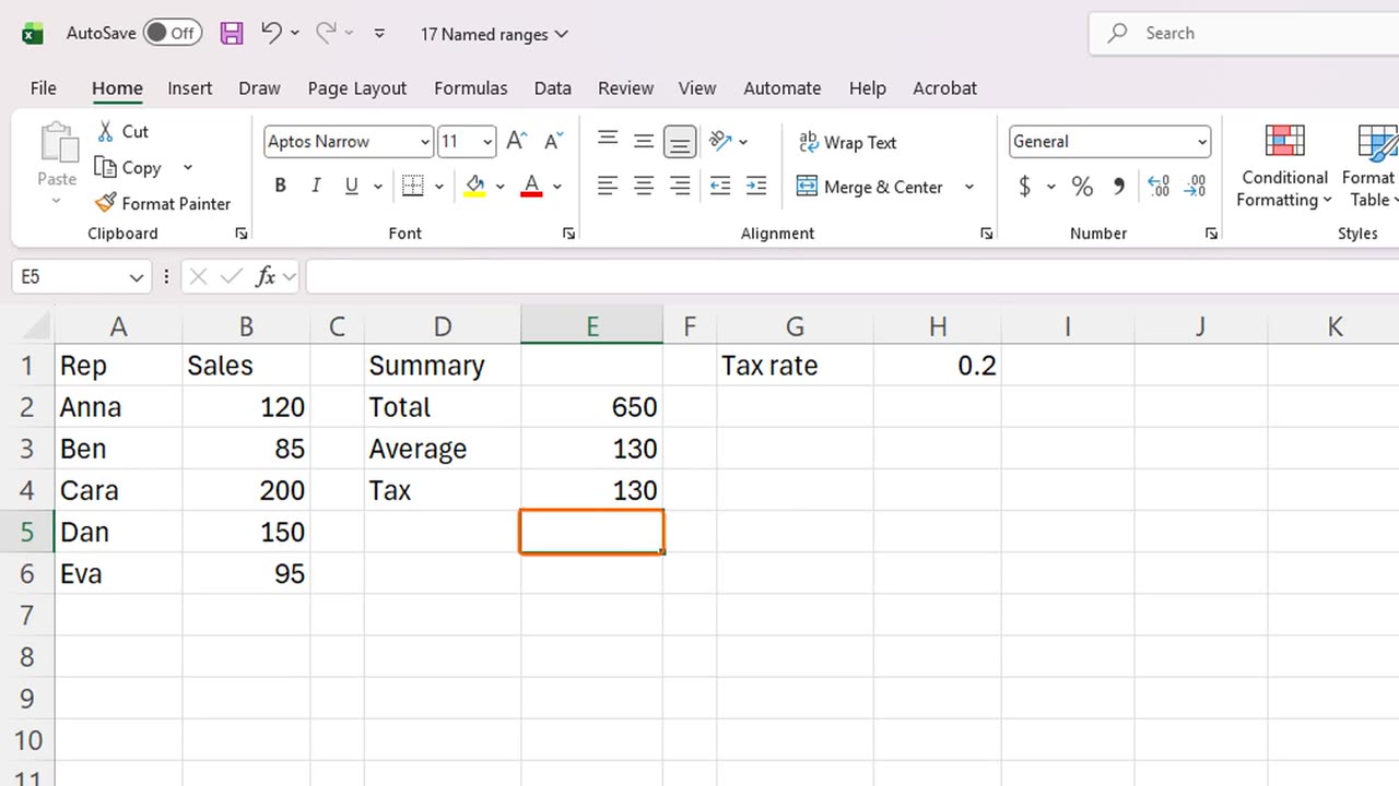
4. Jump to a name
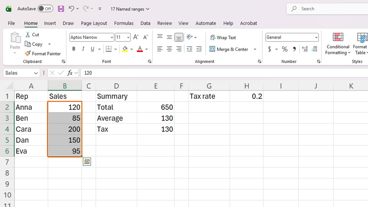
Names also help you move around. Click A1. Then click the Name Box, type Sales, and press Enter.
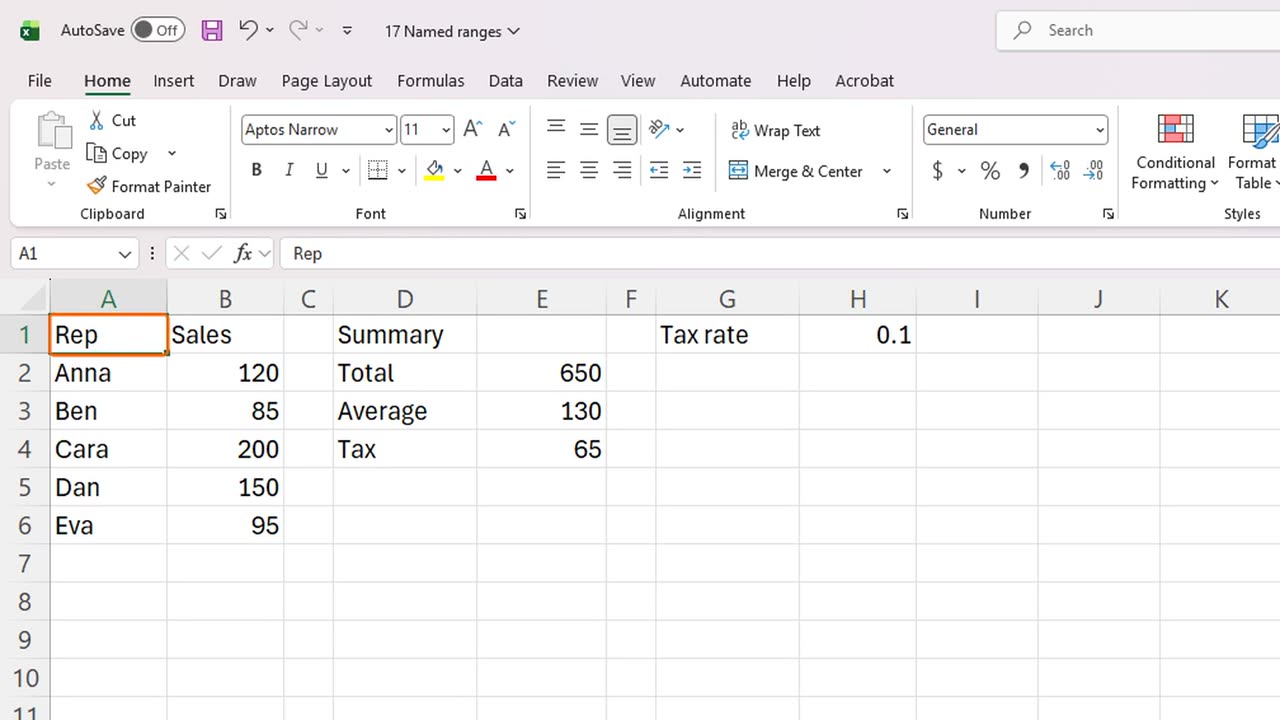
Excel selected the whole Sales range at once. In a big workbook, this is a fast way to jump straight to a table.
You can also open the list of names with the drop down arrow of the Name Box, and see all your names in one place.
5. Easy changes
Names make changes easy. Click H1 and change the tax rate to ten percent, by typing zero point one.
The tax result updated, from one hundred and thirty to sixty five. You changed one cell, and every formula that uses the name followed.
6. Naming rules
There are a few rules for names. They cannot contain spaces, so use one word, or an underscore. They must start with a letter or an underscore. And they cannot look like a cell address, so A1 or B2 are not allowed.
A good name is short and meaningful. Sales and TaxRate are better than X and Number1. Your future self will thank you.
7. Recap
Let's recap. Select a range, type a name in the Name Box, and press Enter. Use the name in formulas. Type a name in the Name Box to jump to it. And follow the naming rules.
Next time, you will learn formula auditing: how to trace where a formula gets its numbers, and how to debug it step by step.
If there is something you want to learn next, write it in the comments. Your requests decide what we teach in the next tutorials. Thanks for watching, and see you in the next one.
← Previous tutorial: XLOOKUP and VLOOKUP in Excel (Easy Lookup Tutorial)
Next tutorial: Excel Formula Auditing: Trace Precedents and Show Formulas →