XLOOKUP and VLOOKUP in Excel (Easy Lookup Tutorial)
Look up values in tables with XLOOKUP and the classic VLOOKUP.
- Intro
- The problem
- XLOOKUP
- When nothing is found
- VLOOKUP
- Which one to use
- Common problems
- Recap
Step by step
1. Intro
Welcome back. In this lesson, you will learn the most famous Excel skill of all: looking up information in a table. You will learn the modern XLOOKUP, and the classic VLOOKUP.
A lookup is like finding a name in a phone book. You give Excel a value to search for, and Excel brings back related information from the same row.
2. The problem
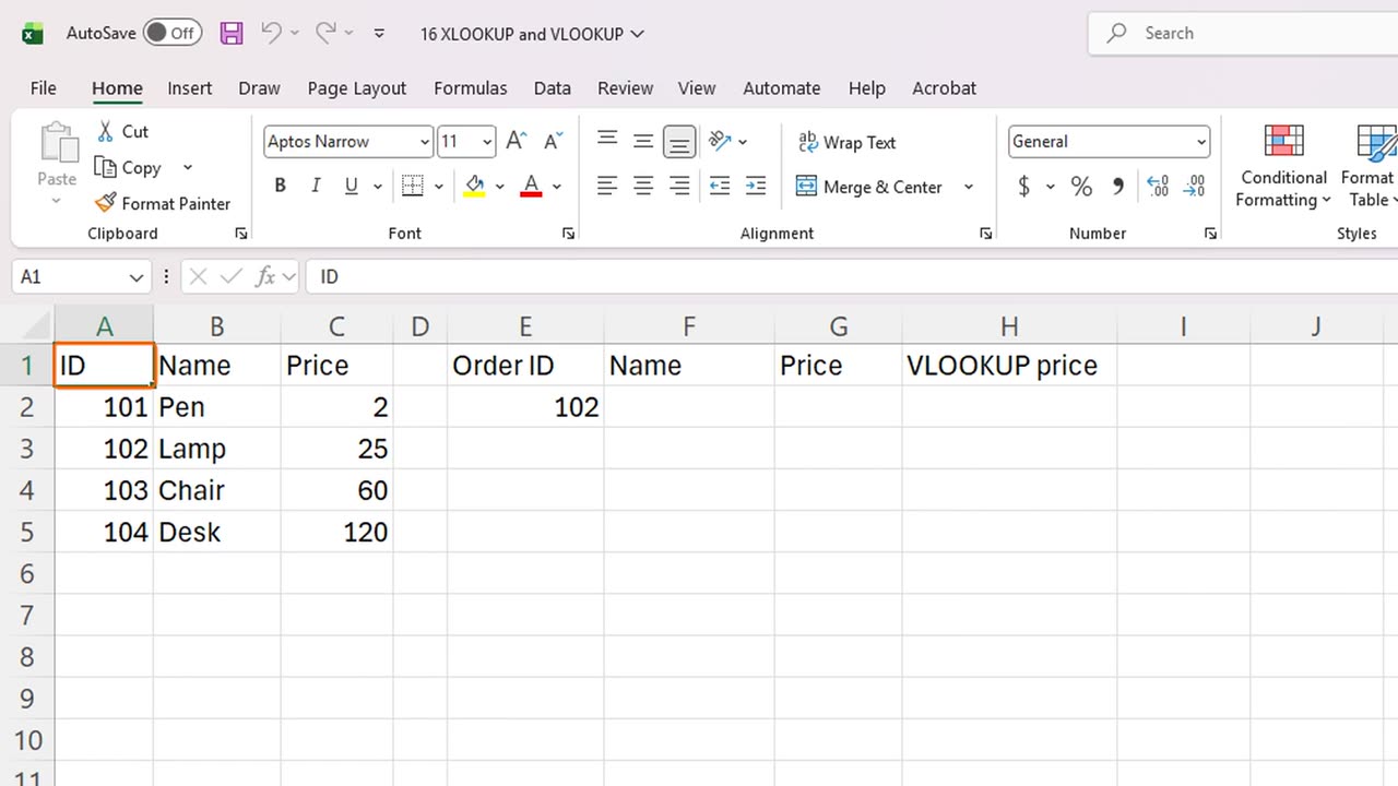
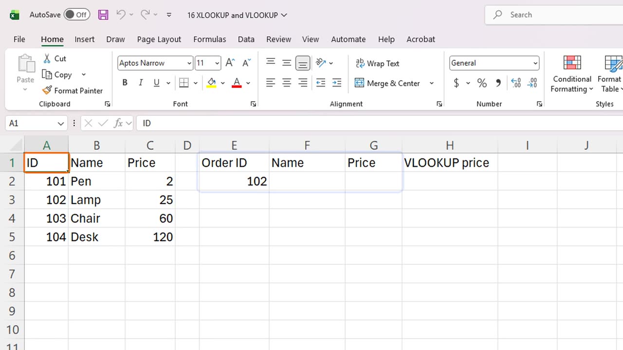
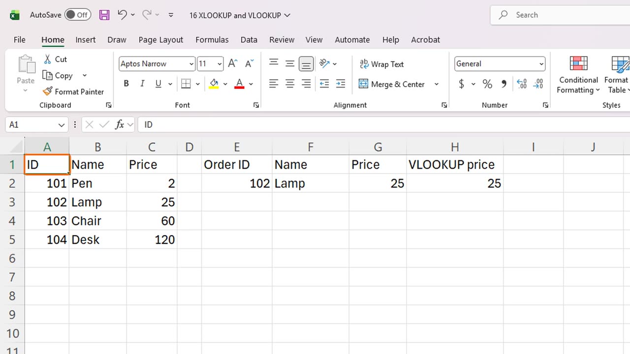
Here is a product table, with an ID, a name and a price. On the right, we have an order, where we only know the product ID. We want Excel to find the name and the price.
3. XLOOKUP
Let's start with XLOOKUP. It has three main parts. What to look for, where to look, and what to return.
Click F2, and type equals XLOOKUP, open bracket, E2, comma, A2 to A5, comma, B2 to B5, close bracket.
Excel looked for the ID in the first column, found it in the second row, and returned the name from the same row: Lamp. The lookup range and the return range must have the same size.
Now the price. In G2, use the same formula, but return column C. Equals XLOOKUP, E2, comma, A2 to A5, comma, C2 to C5.
We have the name and the price, found automatically. Now change the ID. Click E2 and type 104. Both answers update at once.
=XLOOKUP(E2,A2:A5,B2:B5)=XLOOKUP(E2,A2:A5,C2:C5)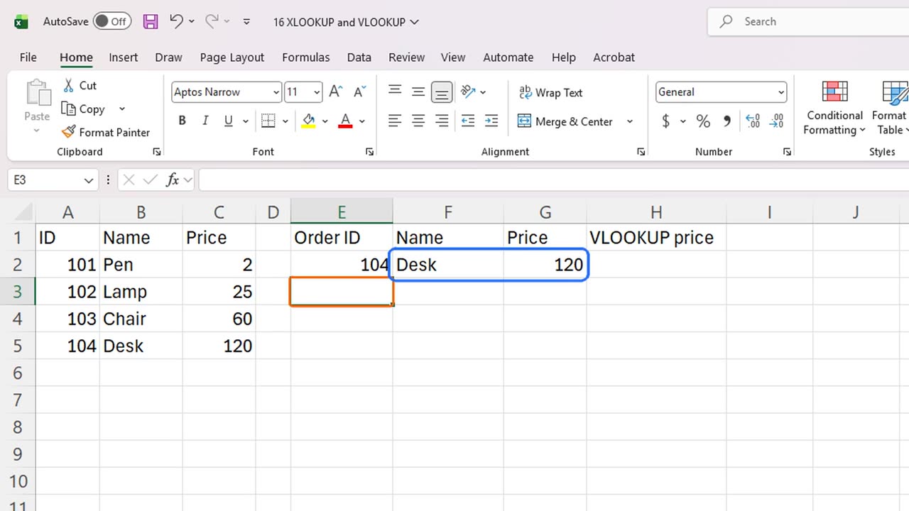
4. When nothing is found
What if the ID does not exist? Type 999 in E2. XLOOKUP shows N slash A, because it found nothing.
XLOOKUP has a built in solution. Add a fourth part: the text to show when nothing is found. Click F2 and add comma, Not found in quotes, at the end.
A friendly message instead of an error. Now put the real ID back: click E2 and type 102.
=XLOOKUP(E2,A2:A5,B2:B5,"Not found")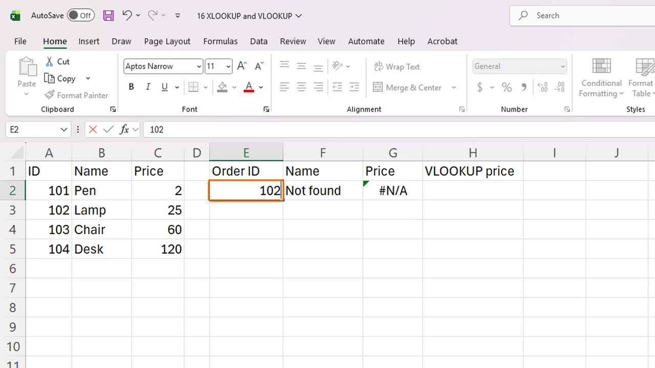
5. VLOOKUP
Now VLOOKUP, the classic. You will meet it in old workbooks everywhere, so you should know how to read it. VLOOKUP has four parts: what to look for, the whole table, which column number to return, and false for an exact match.
Click H2 and type equals VLOOKUP, E2, comma, A2 to C5, comma, 3, comma, FALSE. The 3 means: return the third column of the table.
It returns the same price as XLOOKUP. Always type FALSE at the end. Without it, VLOOKUP does an approximate match, and can give wrong answers.
=VLOOKUP(E2,A2:C5,3,FALSE)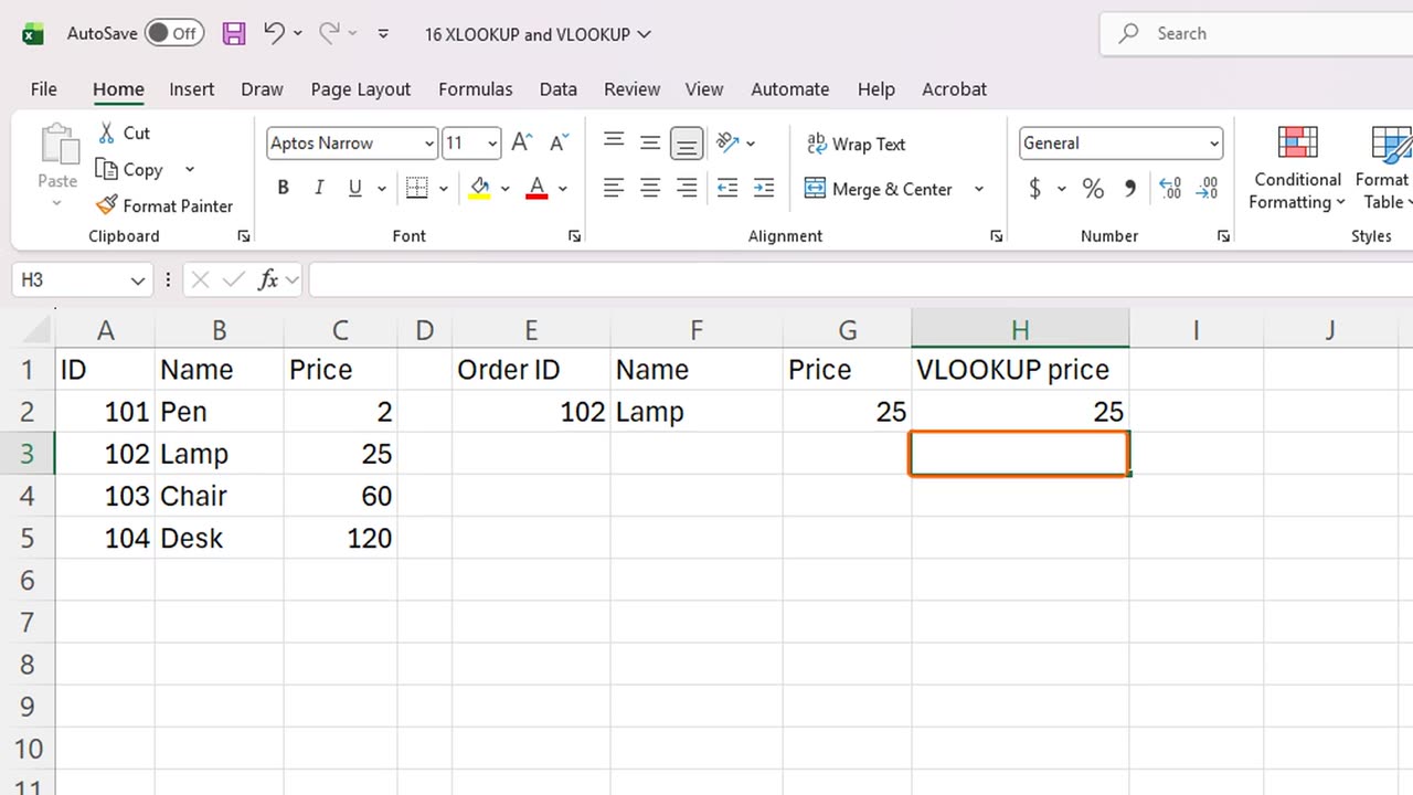
6. Which one to use
So which one should you use? XLOOKUP is easier, it can look to the left, it does not break when you insert columns, and it has the not found message built in. VLOOKUP only looks to the right, and counts columns by number.
If your Excel is older than twenty twenty one, XLOOKUP may not exist, and VLOOKUP is your tool. Otherwise, choose XLOOKUP.
7. Common problems
Here are common problems. A lookup value with a hidden space or a typo gives N slash A. Numbers stored as text do not match real numbers. And the lookup range must contain the value you search for.
8. Recap
Let's recap. A lookup finds related information from a table. XLOOKUP needs what, where and return. VLOOKUP needs the table and a column number, and FALSE. And XLOOKUP can show a message when nothing is found.
Next time, you will learn to give ranges names, which makes your formulas easy to read.
If there is something you want to learn next, write it in the comments. Your requests decide what we teach in the next tutorials. Thanks for watching, and see you in the next one.
← Previous tutorial: Fix Excel Errors: #N/A, #DIV/0!, #REF! and IFERROR
Next tutorial: Excel Named Ranges (Make Formulas Easy to Read) →