Fix Excel Errors: #N/A, #DIV/0!, #REF! and IFERROR
Understand common errors and hide them gracefully with IFERROR.
- Intro
- Divide by zero
- The VALUE error
- The N/A error
- The NAME error
- The REF error
- Error cheat sheet
- IFERROR
- A warning
Step by step
1. Intro
Welcome back. In this lesson, you will learn to read the error messages that Excel shows, understand what each one means, and hide them gracefully with the IFERROR function.
Errors look scary, but they are helpful. Each one is a clue that tells you what went wrong. You will learn five of them: divide by zero, value, N slash A, name, and ref.
2. Divide by zero
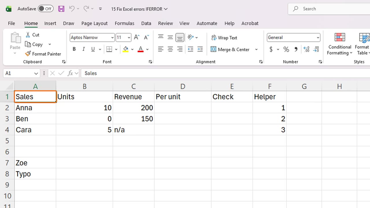
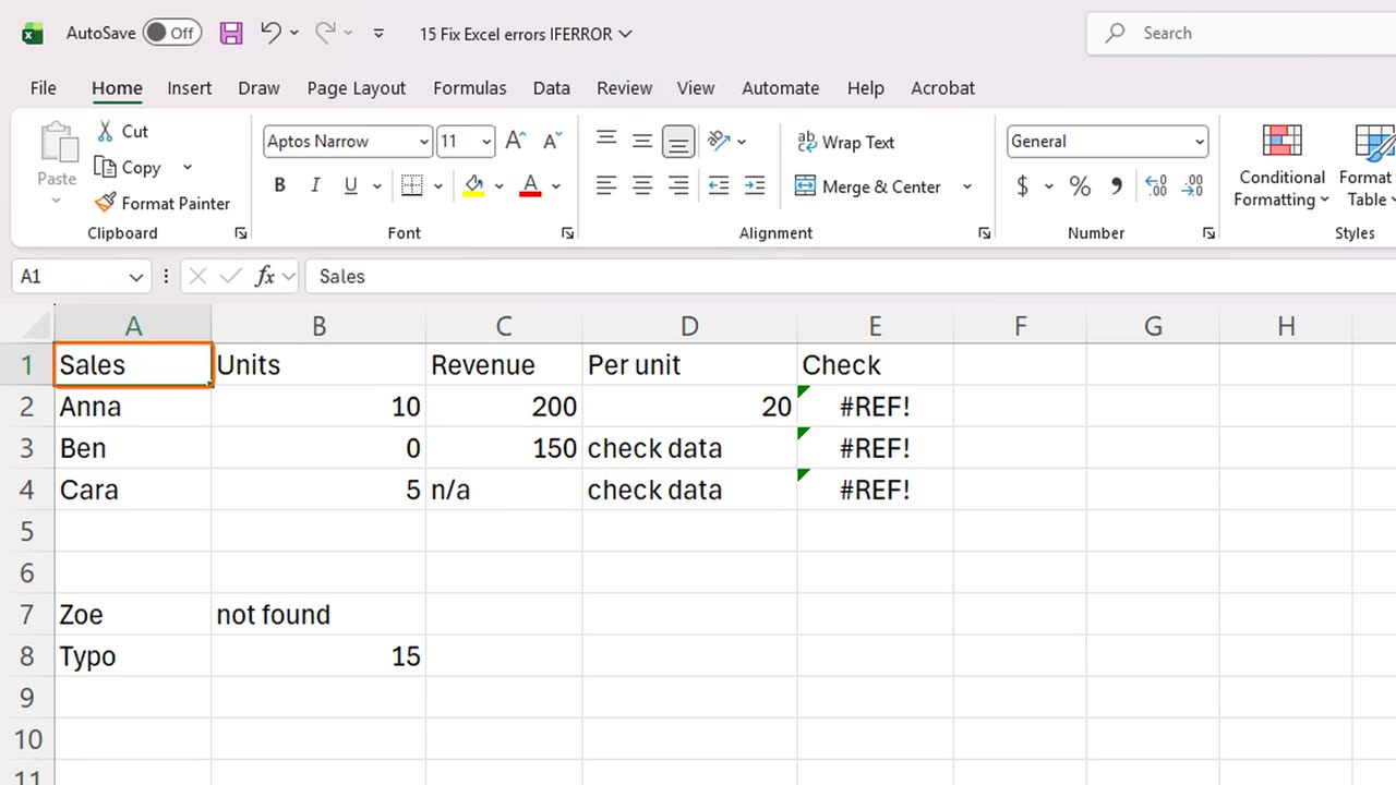
Here is a small table with units and revenue. We want to calculate the revenue per unit. Notice that Ben has zero units, and Cara's revenue contains text, not a number.
Click D2 and type equals C2 divided by B2. Press Enter, and fill the formula down to D4.
The first one works: twenty. But Ben shows hash divide by zero. Excel cannot divide by zero, so it tells you. Check the number you are dividing by.
=C2/B2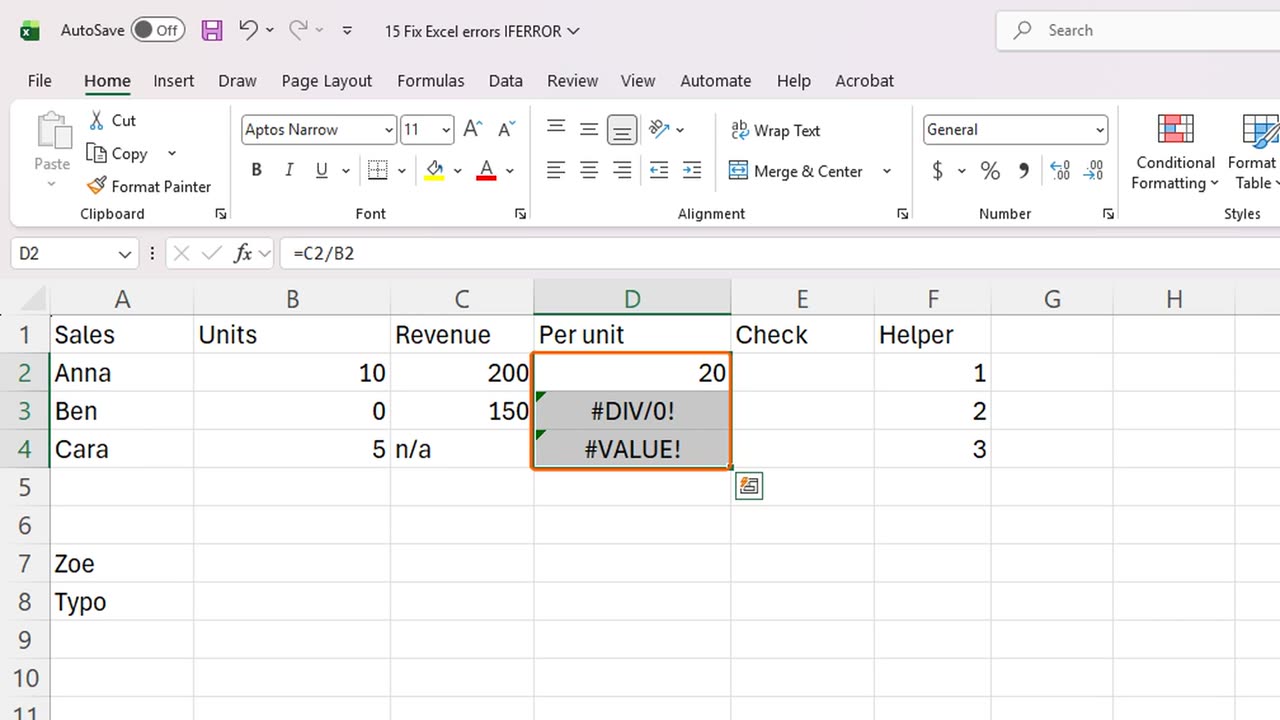
3. The VALUE error
Cara shows hash value. That means a formula received the wrong kind of data, here text where a number was needed. Check for text hiding among your numbers.
4. The N/A error
Now hash N slash A. It means: not available, the thing you are looking for was not found. In B7, we search for Zoe in the table, using VLOOKUP, which you will learn in a later lesson.
Zoe is not in the table, so Excel shows N slash A. Often, the name is there but has a typo or a hidden space. Always check the spelling first.
=VLOOKUP(A7,A2:C4,2,FALSE)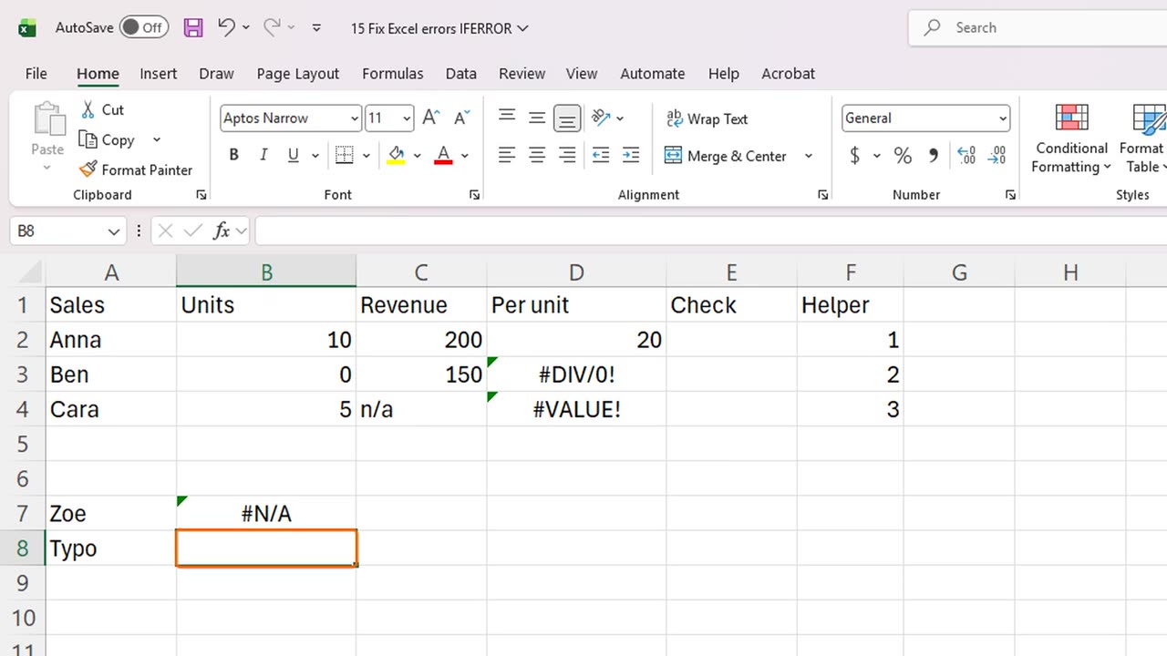
5. The NAME error
Next, hash name. It means Excel does not recognize a word in your formula. In B8, we type SUMM, with two Ms, by mistake.
Excel shows hash name. A misspelled function name is the usual cause. Fix the spelling, and it works. Retype it correctly: equals SUM, B2 to B4.
=SUMM(B2:B4)=SUM(B2:B4)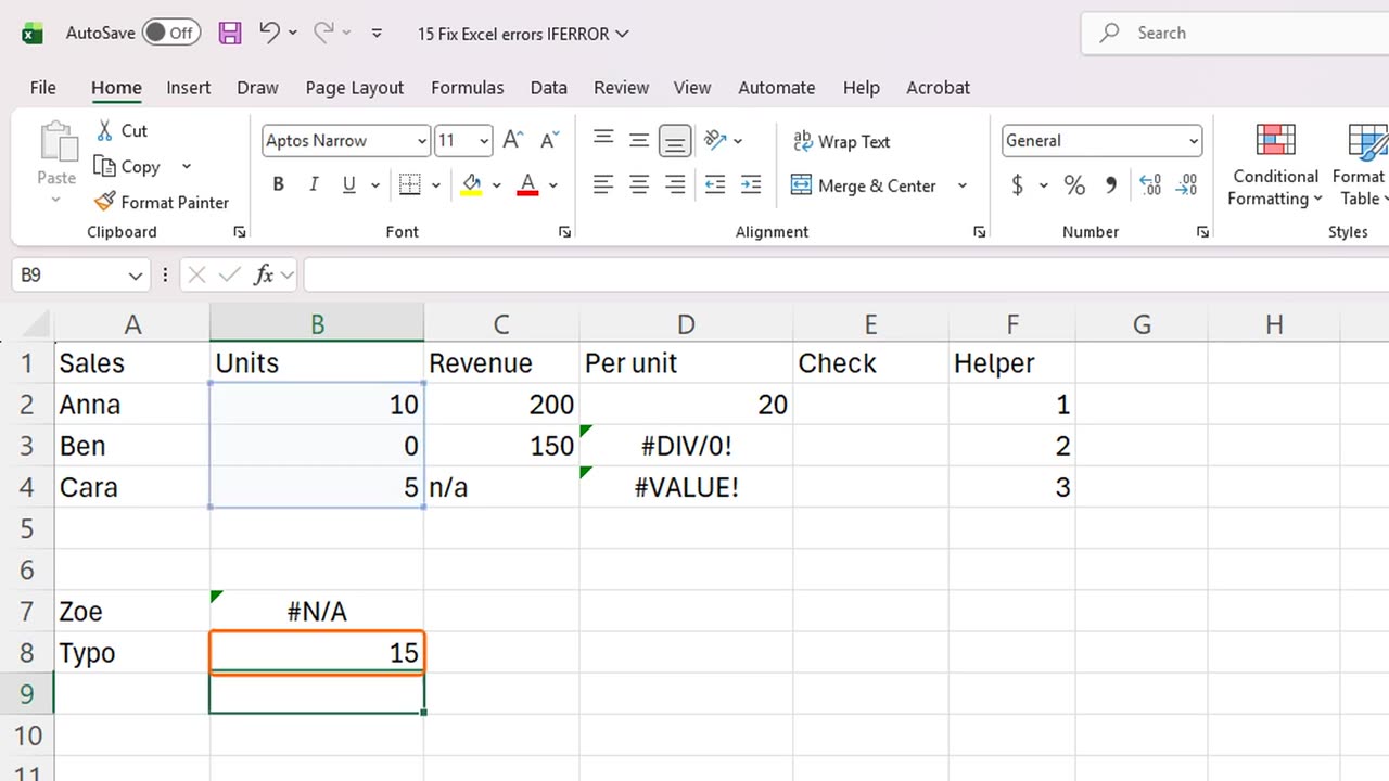
6. The REF error
The last error is hash ref. It means a formula points to a cell that no longer exists. To see it, in column E, we write a formula that uses the helper numbers in column F.
Now delete column F, which the formulas depend on. Click the column F header, and press Control and the minus key.
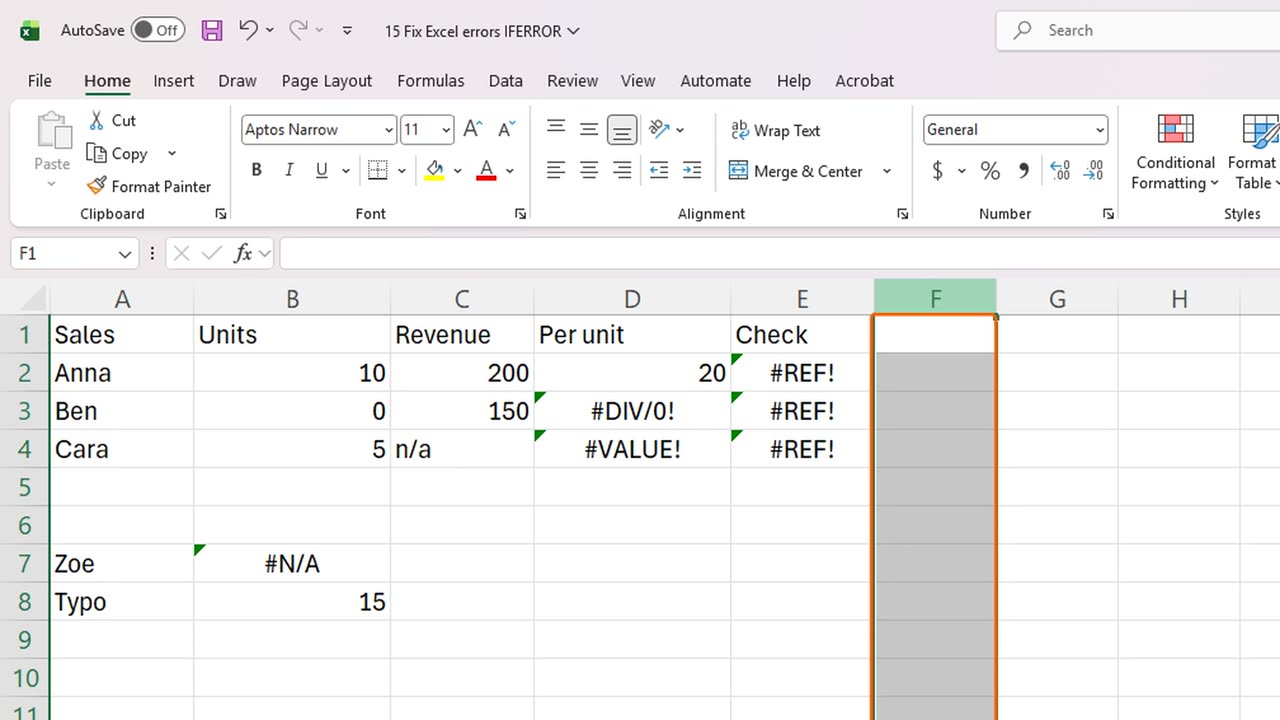
Column E now shows hash ref. The cells that the formula needed are gone. If you see this right after deleting something, press Control Z to undo the delete.
=F2*2Shortcut: Ctrl + -
7. Error cheat sheet
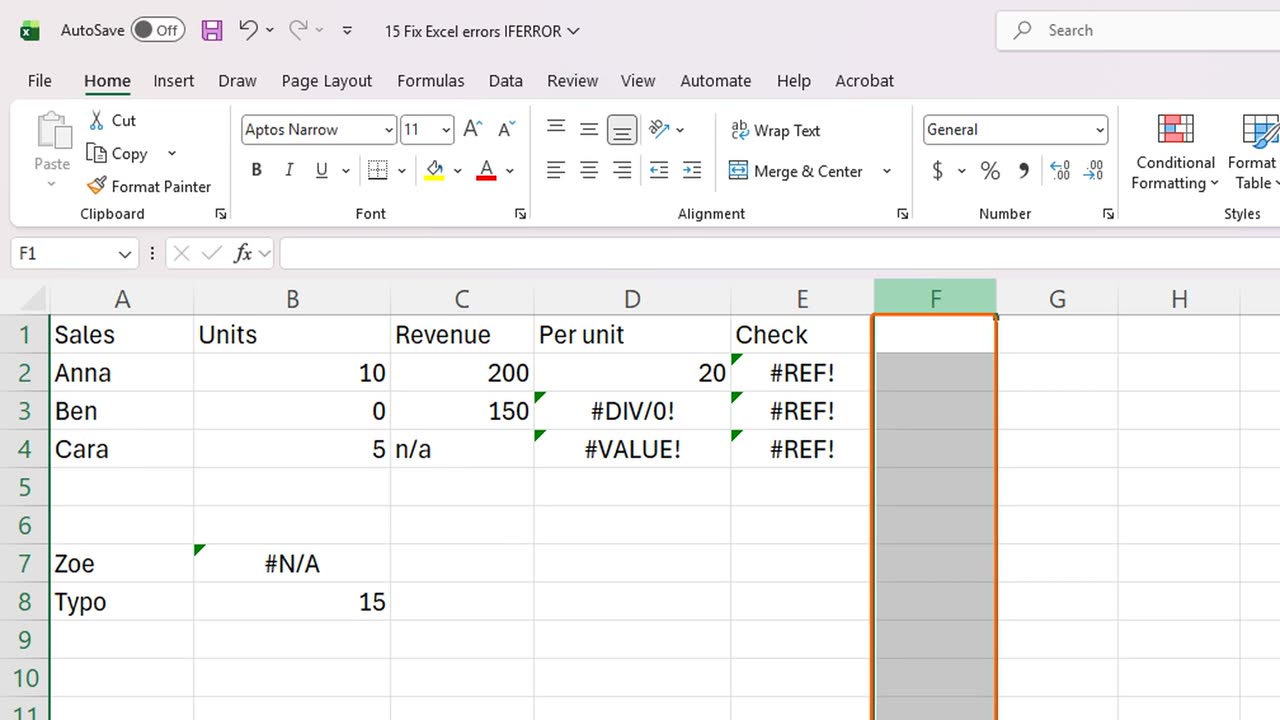
Let's recap the five errors. Divide by zero: dividing by zero or an empty cell. Value: wrong type of data. N slash A: not found. Name: unknown word. And ref: a deleted cell.
8. IFERROR
Sometimes an error is expected, and you just want a clean report. That is the job of IFERROR. It takes two things: the formula to try, and what to show if it fails.
Click D2 and type equals IFERROR, open bracket, C2 divided by B2, comma, check data in quotes, close bracket. Fill it down.
The errors are replaced by a friendly message, and the good result, twenty, is untouched.
Do the same for the lookup. In B7, wrap the VLOOKUP in IFERROR, and show not found in quotes.
=IFERROR(C2/B2,"check data")=IFERROR(VLOOKUP(A7,A2:C4,2,FALSE),"not found")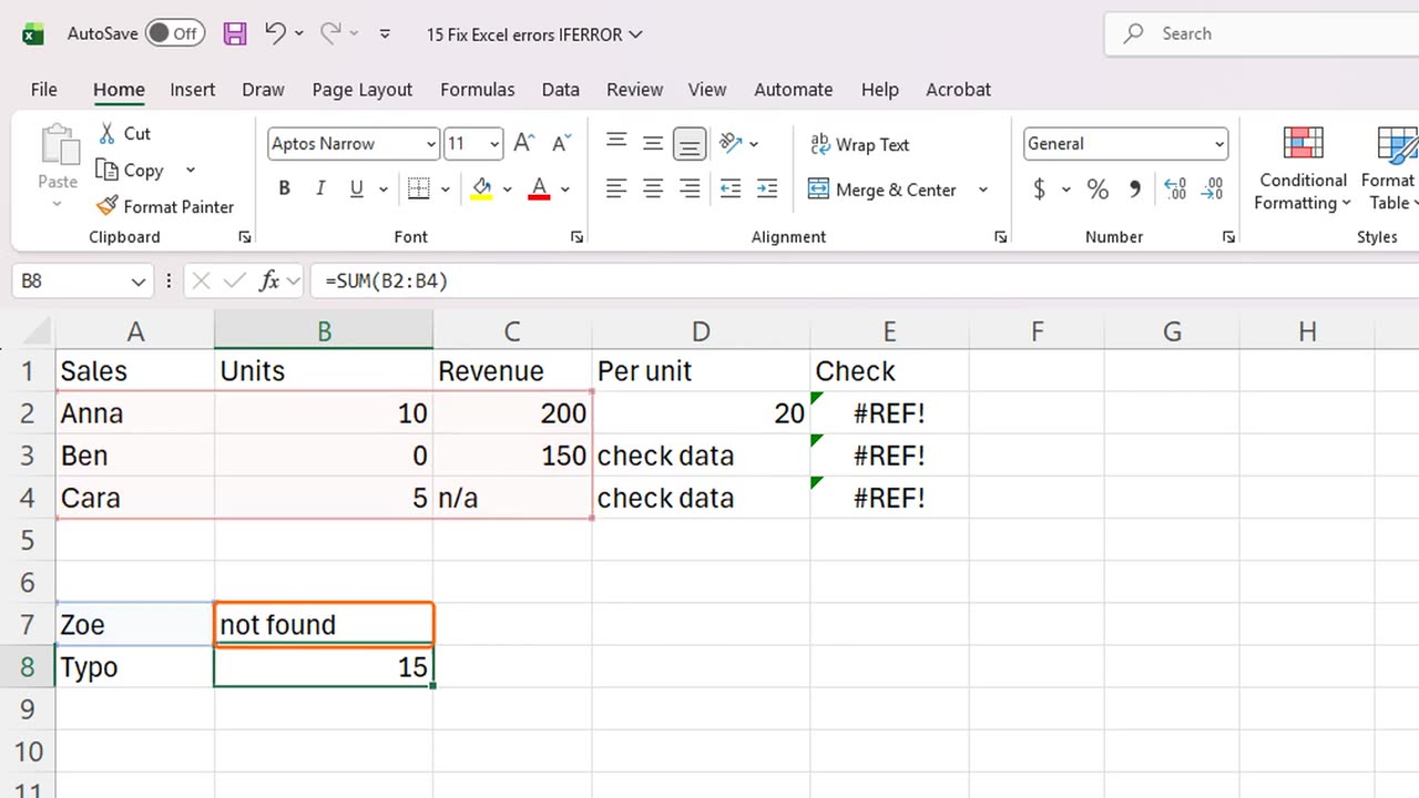
9. A warning
A warning: IFERROR hides every error, including real mistakes. Use it when you expect a certain error, and fix real problems first. Never hide an error you do not understand.
Next time, you will meet the lookup functions: XLOOKUP and VLOOKUP.
If there is something you want to learn next, write it in the comments. Your requests decide what we teach in the next tutorials. Thanks for watching, and see you in the next one.
← Previous tutorial: Excel Date Functions: TODAY, NOW, DATEDIF, EOMONTH
Next tutorial: XLOOKUP and VLOOKUP in Excel (Easy Lookup Tutorial) →