Rows, Columns and Borders in Excel (Resize, Insert, Delete)
Resize, insert, delete, hide rows and columns, autofit widths and add borders.
- Intro
- Resize columns
- Resize rows
- Insert and delete
- Hide and unhide
- Faster editing
- Borders
- Recap
Step by step
1. Intro
Welcome back. In this lesson, you will learn to resize, insert, delete and hide rows and columns, and to add borders to your tables.
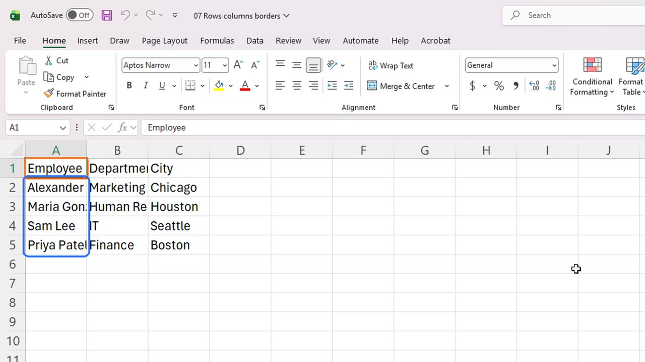
We have a small employee list. Look at the first column: the names are cut off, because the column is too narrow for them.
2. Resize columns
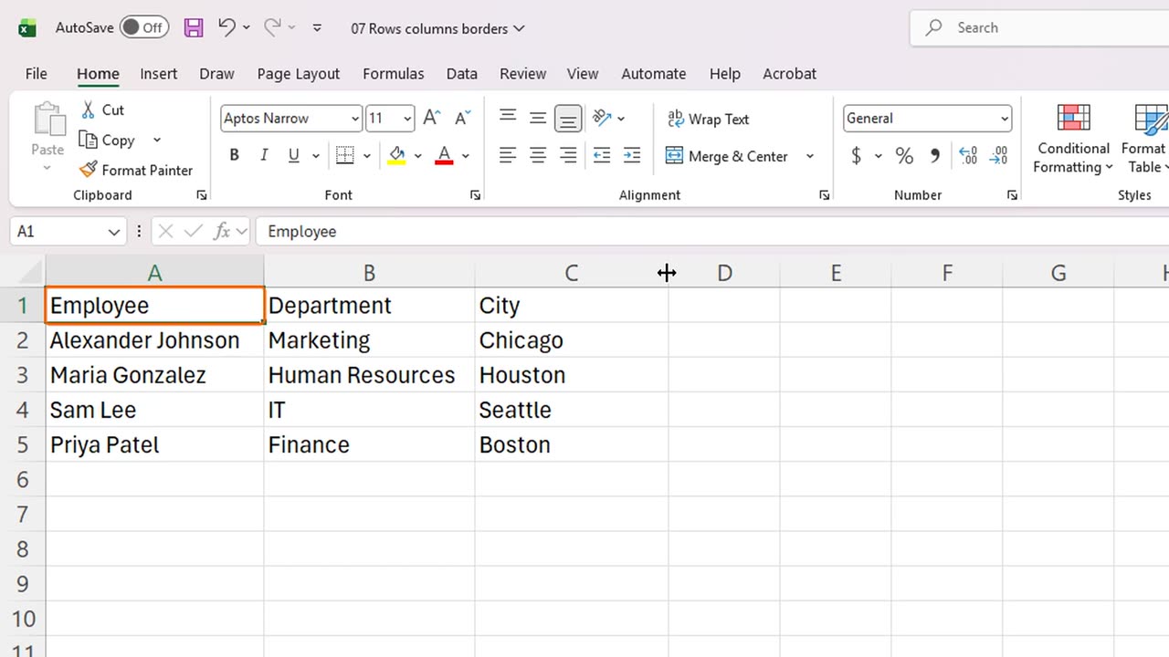
The fastest fix is AutoFit. Point at the line between the column letters A and B, and double-click.
The column grew to fit the longest name. Do the same for column B.
You can also drag the line to set any width you like. Let's make column C wider.
3. Resize rows
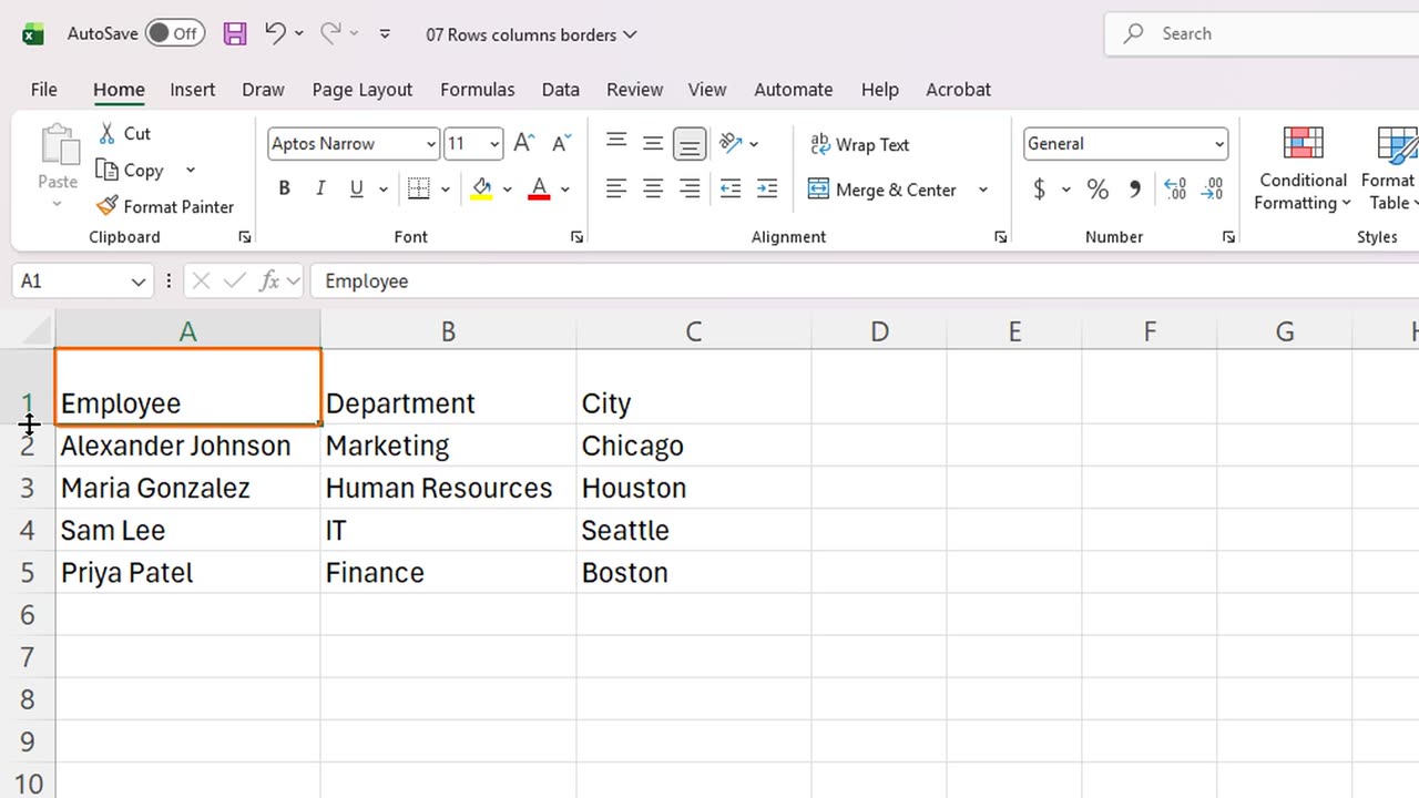
Rows work the same way. Drag the line under row number one to make the header row taller.
4. Insert and delete
Next, inserting. Suppose we forgot an employee. Click the number of row three to select the whole row.
On the Home tab, click Insert. A new empty row appears above row three, and the rows below move down.
To delete the row again, with it still selected, click Delete.
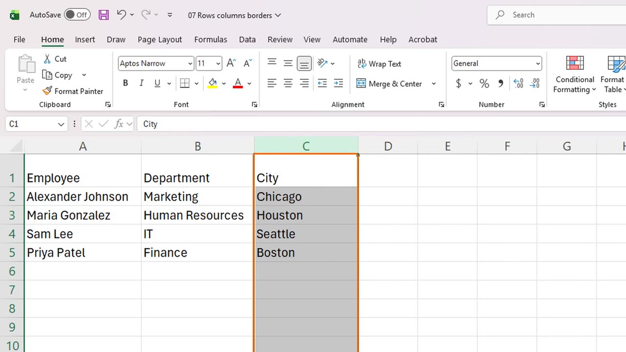
Columns work the same way. Select column C by clicking its letter, then click Insert, and delete it again.
5. Hide and unhide
Sometimes you do not want to delete, only to hide. Select rows three to four, and press Control and nine.
Look at the row numbers: they jump from two to five. The data is still there, just hidden.
To show them again, select the rows around the hidden ones, rows two to five, and press Control, Shift and nine.
6. Faster editing
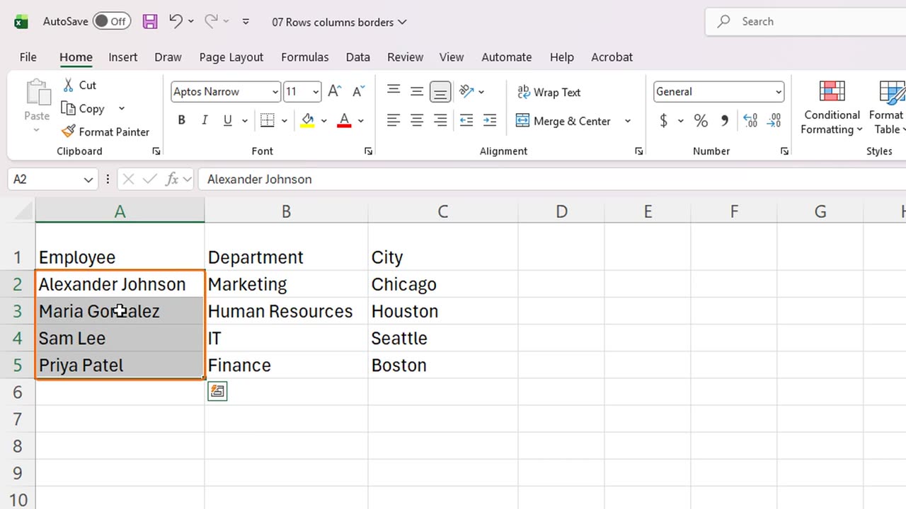
You can select several rows at once by dragging across their numbers. Here are rows two to four.
Click Insert, and Excel inserts three rows at once. Then click Delete to remove them again.
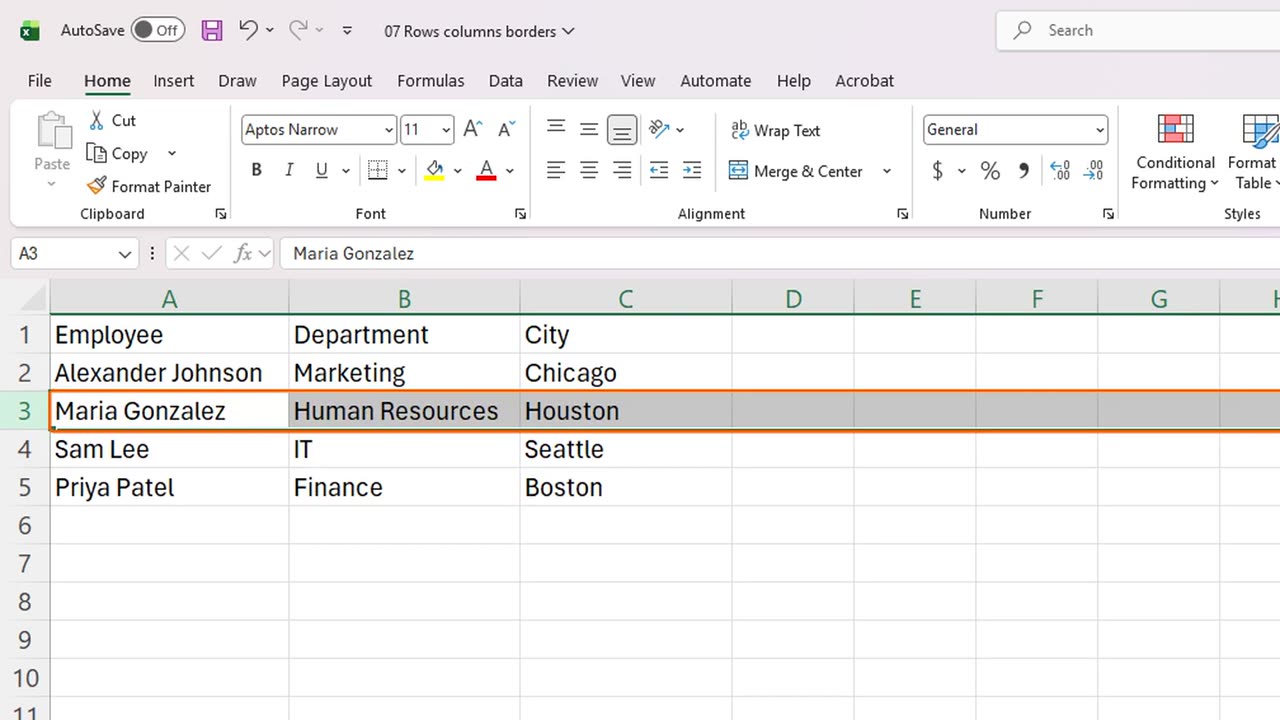
Here are keyboard shortcuts. Click a cell and press Shift and Space to select its row, or Control and Space to select its column.
With a row selected, Control Shift and the plus key inserts a new row, and Control and the minus key deletes it.
Rows can AutoFit too. Double-click the line under a row number, and the row fits its content. Let's fix the tall header row.
Shortcut: Ctrl + -
7. Borders
Now borders. The faint gray gridlines you see on screen do not print. Real borders do.
Select the whole table, A1 to C5.
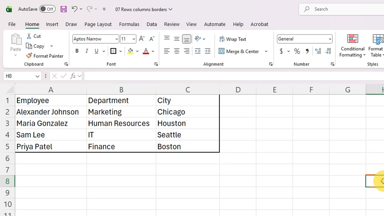
The Borders button is in the Font group. For speed, press Alt, then H, B, and A, which means All Borders.
Every cell now has a border. The same menu has more styles, such as outside borders, thick borders and bottom borders.
Let's try other border styles. Select the table again. Alt, H, B, N removes all borders.
Alt, H, B, S draws a border around the outside of the selection.
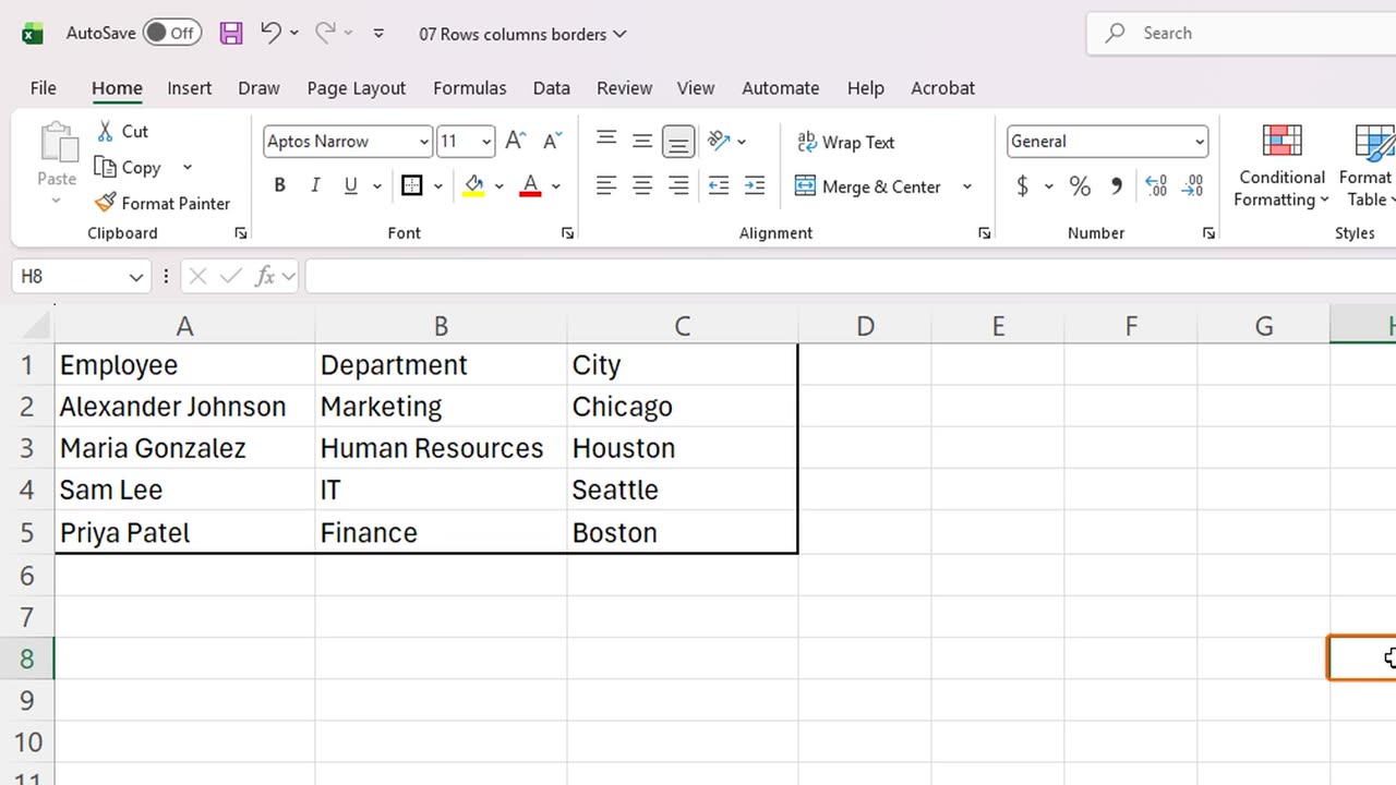
And Alt, H, B, T draws a thick box around it, which is great for totals and headers.
8. Recap
Let's recap. Double-click the line between two column letters to AutoFit, or drag it to choose a width.
Select a row or column and use Insert and Delete on the Home tab. Hide with Control nine, and show again with Control Shift nine.
Add borders with Alt, H, B, A. Next time, you will customize the Quick Access Toolbar and the ribbon.
Thanks for watching, and see you in the next lesson.
← Previous tutorial: Format Text, Numbers and Dates in Excel
Next tutorial: Customize the Excel Quick Access Toolbar and Ribbon →