Format Text, Numbers and Dates in Excel
Bold, colors, alignment, number formats, currency, percent and date formats.
- Intro
- Font and color
- Alignment
- Number formats
- Dates
- Wrap, paint and merge
- Quick wins
- Recap
Step by step
1. Intro
Welcome back. In this lesson, you will make your data look professional: bold headers, colors, alignment, and number formats for currency, percent and dates.
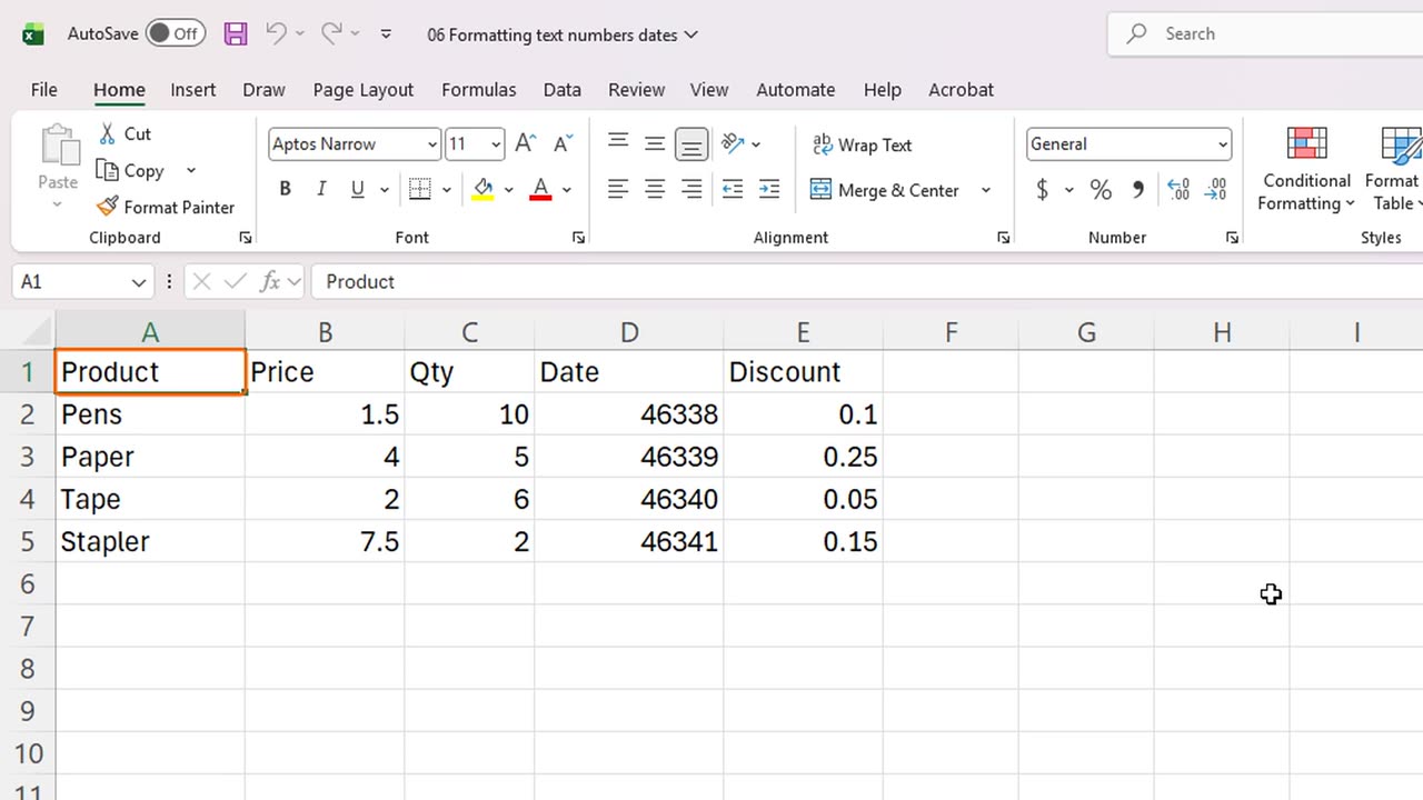
Here is a small sales table. It is correct, but it is plain and hard to read. The prices have no currency, the discounts are decimals, and the dates are strange numbers.
2. Font and color
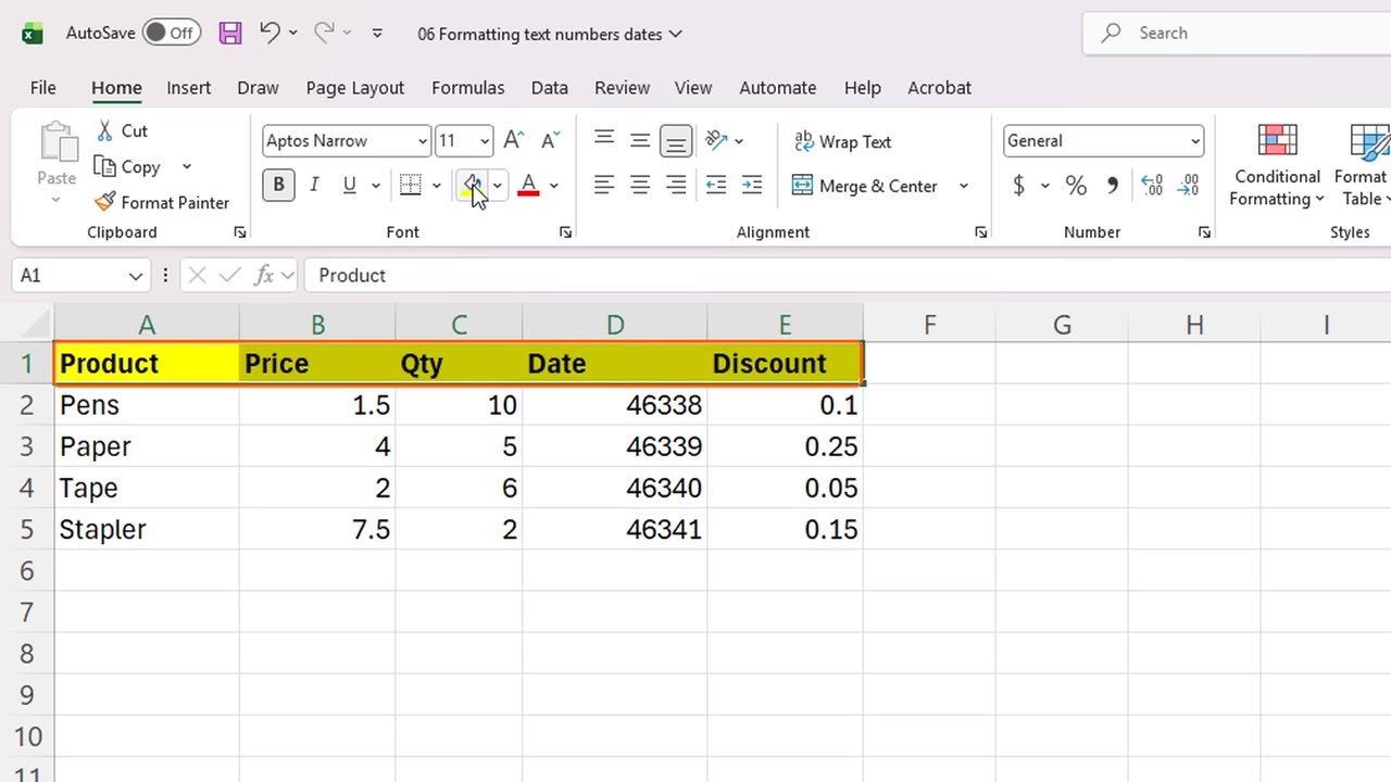
Let's start with the header. Drag across A1 to E1 to select it.
On the Home tab, in the Font group, click Bold. Or press Control and B.
Next, the fill color button, the paint bucket, adds a background color. Click it.
The little arrow next to it opens a palette of more colors, and the letter A button next to that changes the font color.
3. Alignment
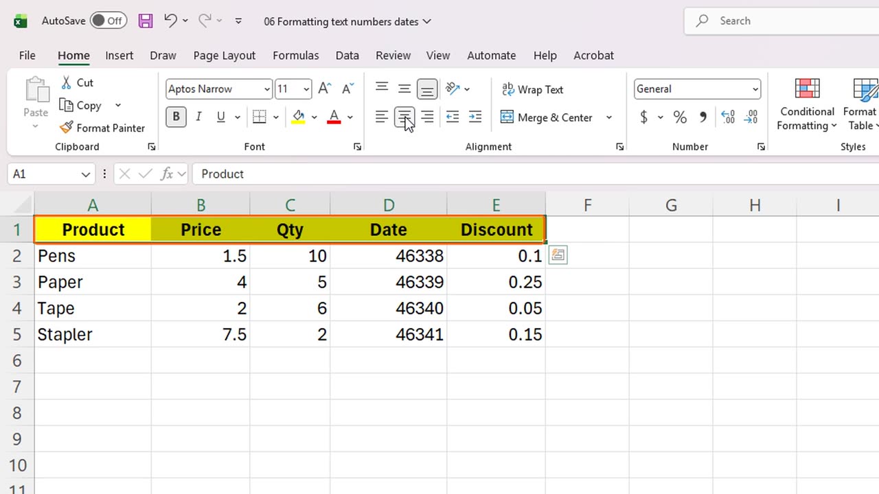
Now alignment. With the header still selected, click Center, to put the text in the middle of the cells.
The other buttons align text to the left or to the right, and the Wrap Text button breaks long text into several lines inside a cell.
4. Number formats
Now numbers. Select the prices, B2 to B5.
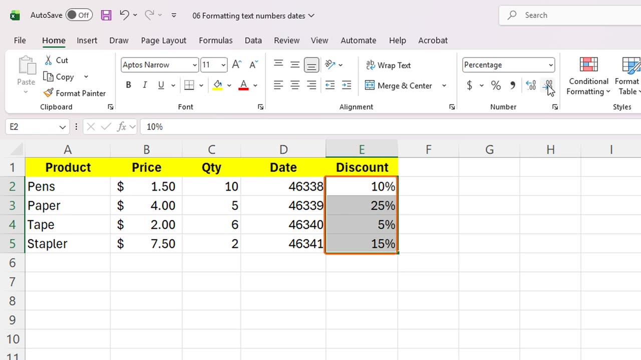
Click the dollar sign button. The numbers become currency, with a dollar symbol and two decimals.
Important: the number inside the cell did not change. Only its appearance did. Formatting never changes the real value.
Now the discounts, E2 to E5. These are decimals, like zero point one. Select them.
Click the percent button, and zero point one becomes ten percent.
The two buttons with the arrows add or remove decimal places. Click Increase Decimal once, then Decrease Decimal to go back.
5. Dates
Finally, the dates. Excel stores a date as a number, which is why we see these big values. Select D2 to D5.
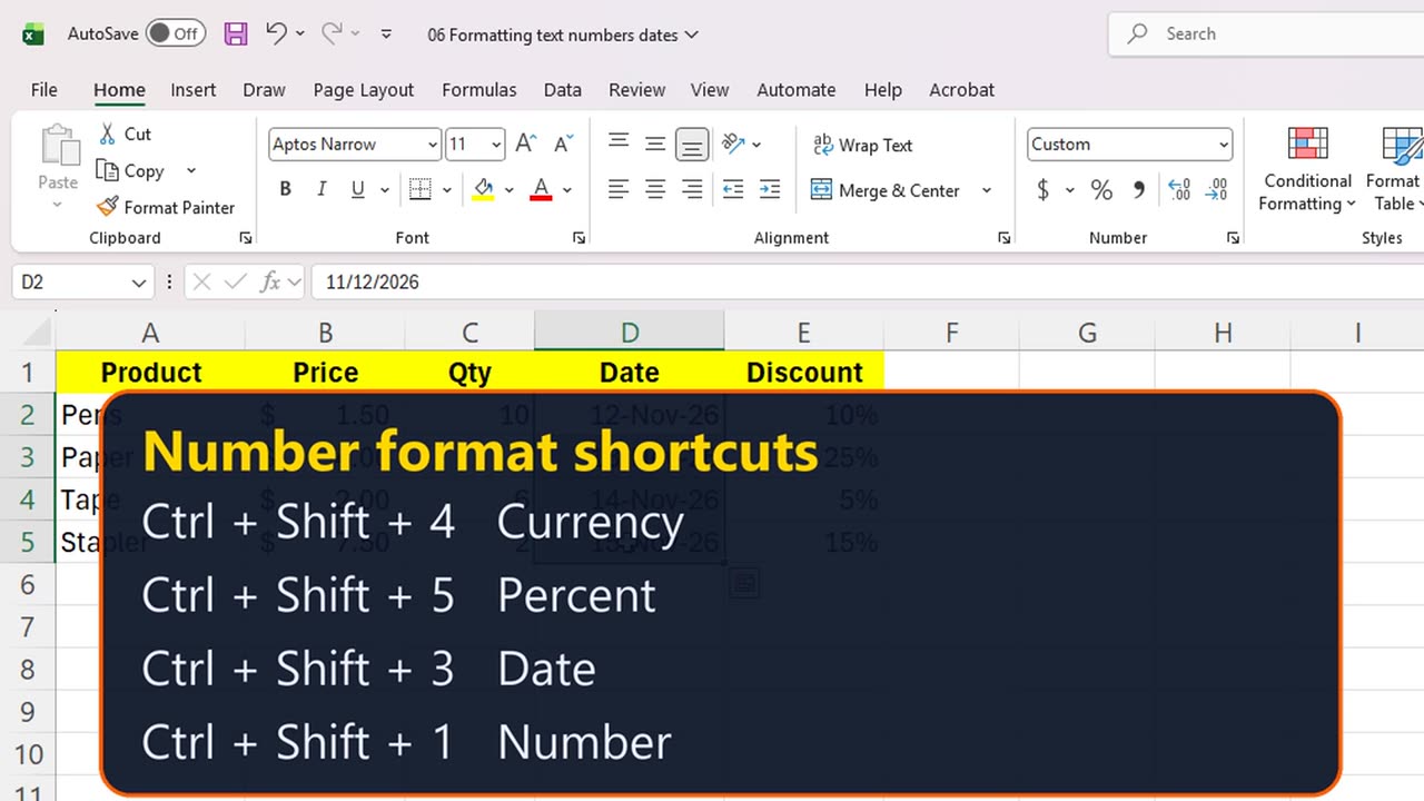
Press Control, Shift and three. Now the numbers show as proper dates.
These shortcuts exist for the other formats too: Control Shift four for currency, and Control Shift five for percent.
Shortcut: Ctrl + Shift + 3
6. Wrap, paint and merge
Now a few more tools. Long text spills over into the cells next to it. Click A9 and type a short note.
Select the cell and click Wrap Text. The text now stays inside the cell, on several lines, and the row grows to fit.
Next, a title for our table. Type Sales report in A7.
Format Painter copies the look of one cell to another. Select the formatted header, click Format Painter, then drag over the title row.
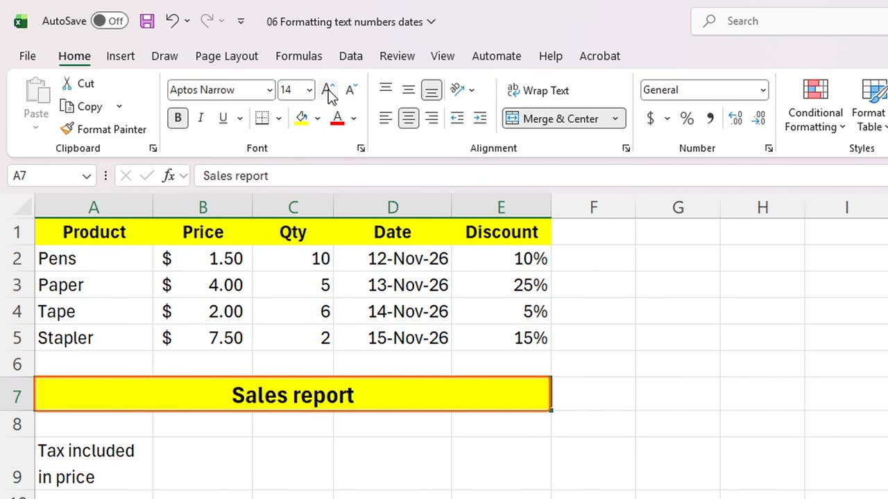
Now, with the title row selected, click Merge and Center. The five cells become one, and the title sits in the middle.
Finally, the letter A with the up arrow makes the font bigger. Click it twice for a real title.
To remove formatting, use the Clear button in the Editing group, then Clear Formats. The data stays, and only the look disappears.
The Number group also has a drop-down box with more formats, such as Long Date, Time and Fraction.
7. Quick wins
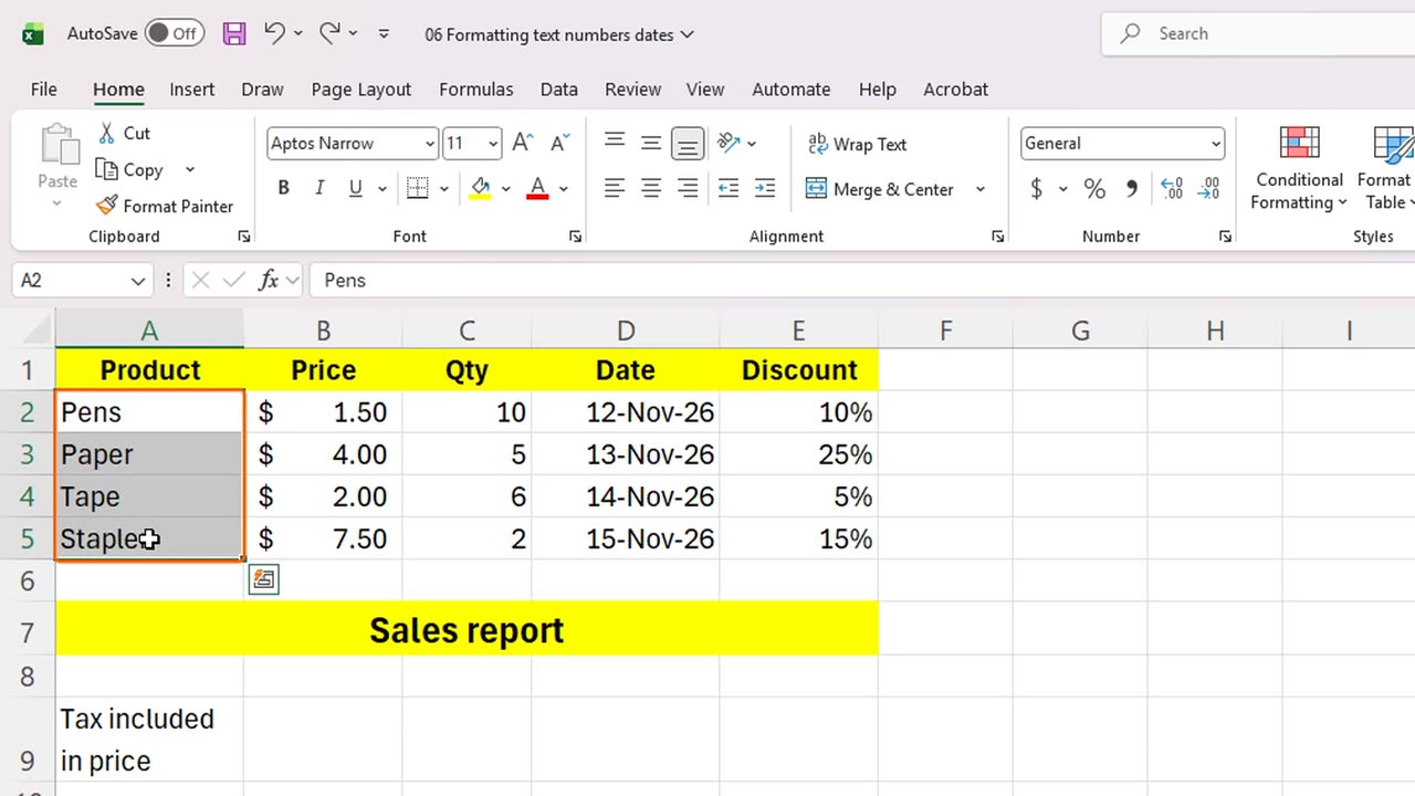
Let's polish the first column. Select the product names and press Control and I for italics.
If you do not like a change, press Control and Z to undo it, just like in any other program.
8. Recap
Let's recap. Bold, fill color, font color and alignment live in the Font and Alignment groups of the Home tab.
Number formats change how values look, not what they are. Use currency, percent and date formats, and the keyboard shortcuts to be faster.
Next time, you will learn to work with rows, columns and borders.
Thanks for watching, and see you in the next lesson.
← Previous tutorial: Your First Excel Formulas (Beginner Tutorial)
Next tutorial: Rows, Columns and Borders in Excel (Resize, Insert, Delete) →