Your First Excel Formulas (Beginner Tutorial)
Start every formula with =, add, subtract, multiply and divide, use cell references and watch a formula update.
- Intro
- The golden rule
- Operators
- Cell references
- Copy a formula
- A grand total
- Handy formula tools
- Recap
Step by step
1. Intro
Welcome back. In this lesson, you will write your first Excel formulas. This is where Excel starts to feel like magic.
You will learn the golden rule of formulas, the four basic operators, cell references, and how to copy a formula down a whole column.
2. The golden rule
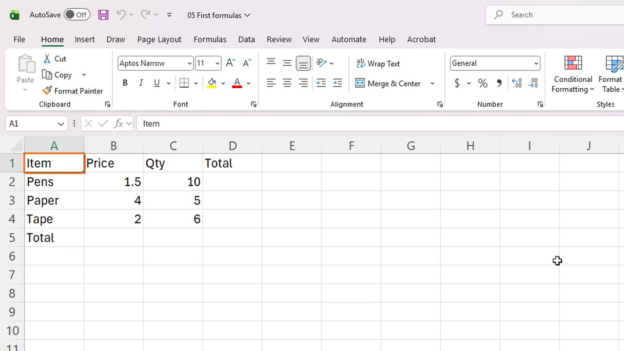
Here is a small shop list with a price and a quantity for each item. We want the total for every row.
The golden rule is this: every formula starts with an equals sign. Without it, Excel treats your entry as plain text.
Click D2, the total for the pens. Type equals, B2, star, C2.
The star means multiply. While you type, Excel colors the cells that the formula uses. Press Enter.
The cell shows the result, fifteen. Select D2 again, and look at the formula bar. The formula is still there.
A tip if your Excel is in another language: function names may be translated, but the equals sign and the operators are exactly the same.
=B2*C2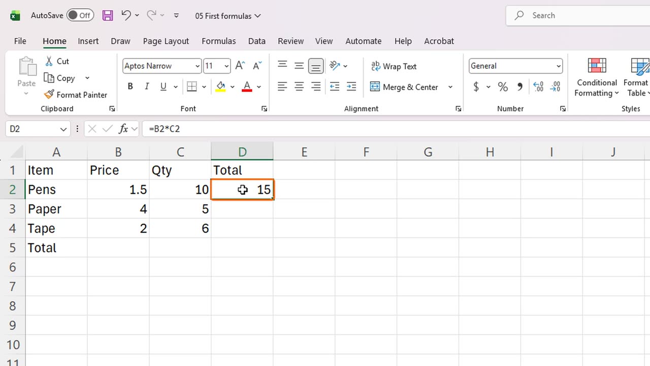
3. Operators
Excel has four basic operators: plus to add, minus to subtract, star to multiply, and slash to divide.
Let's try them in column F. Type equals five plus three.
Equals ten minus four. Equals six star seven. Equals twenty slash four.
And two to the power of three, using the caret symbol.
Excel follows the order of operations: multiplication before addition. Equals two plus three star four gives fourteen.
Use parentheses to change the order. Equals open bracket two plus three close bracket, star four, gives twenty.
=5+3=10-4=6*7=20/4=2^3=2+3*4=(2+3)*4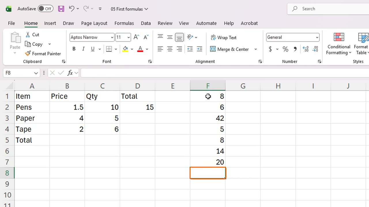
4. Cell references
Now the real power: cell references. Our formula in D2 uses B2 and C2, not fixed numbers.
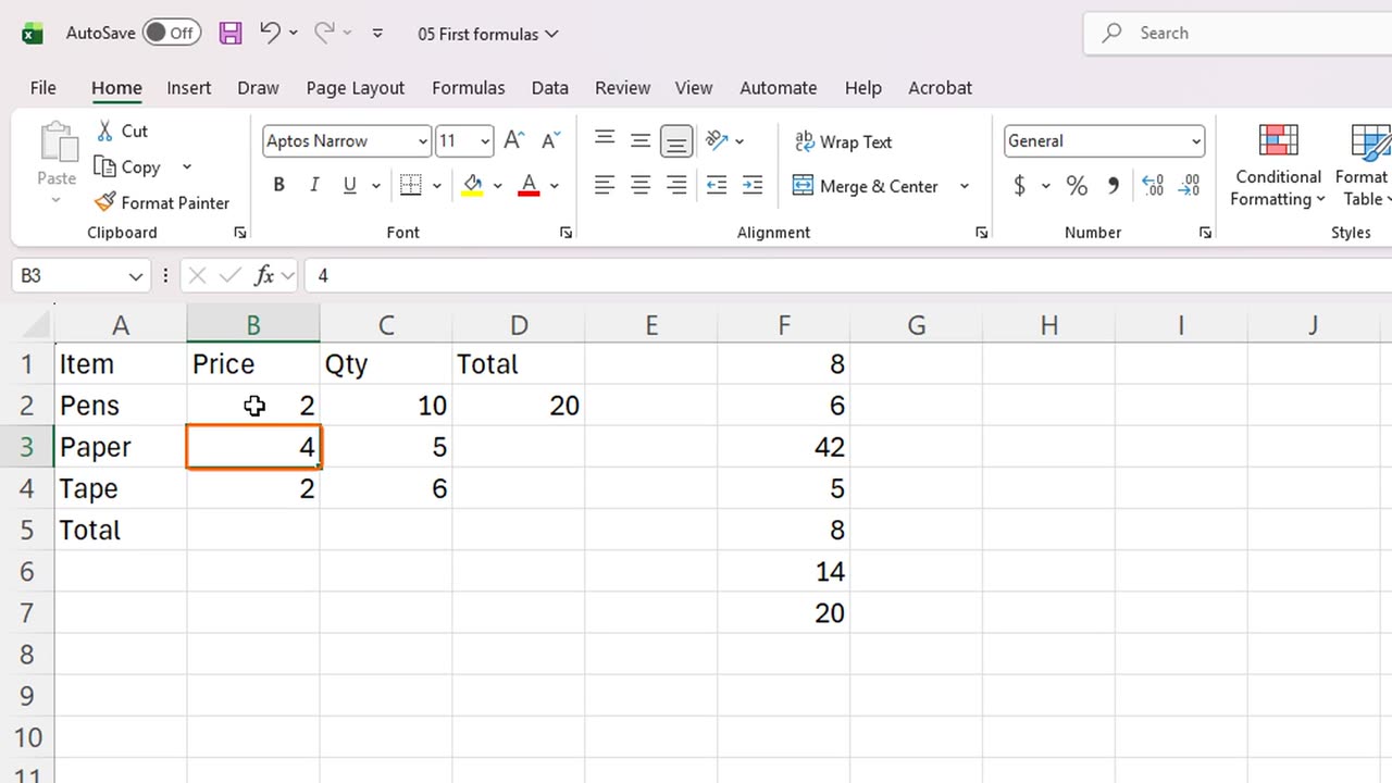
Let's change the price of the pens. Click B2 and type two, then press Enter.
The total in D2 updated by itself. A formula always recalculates when the numbers it points to change.
5. Copy a formula
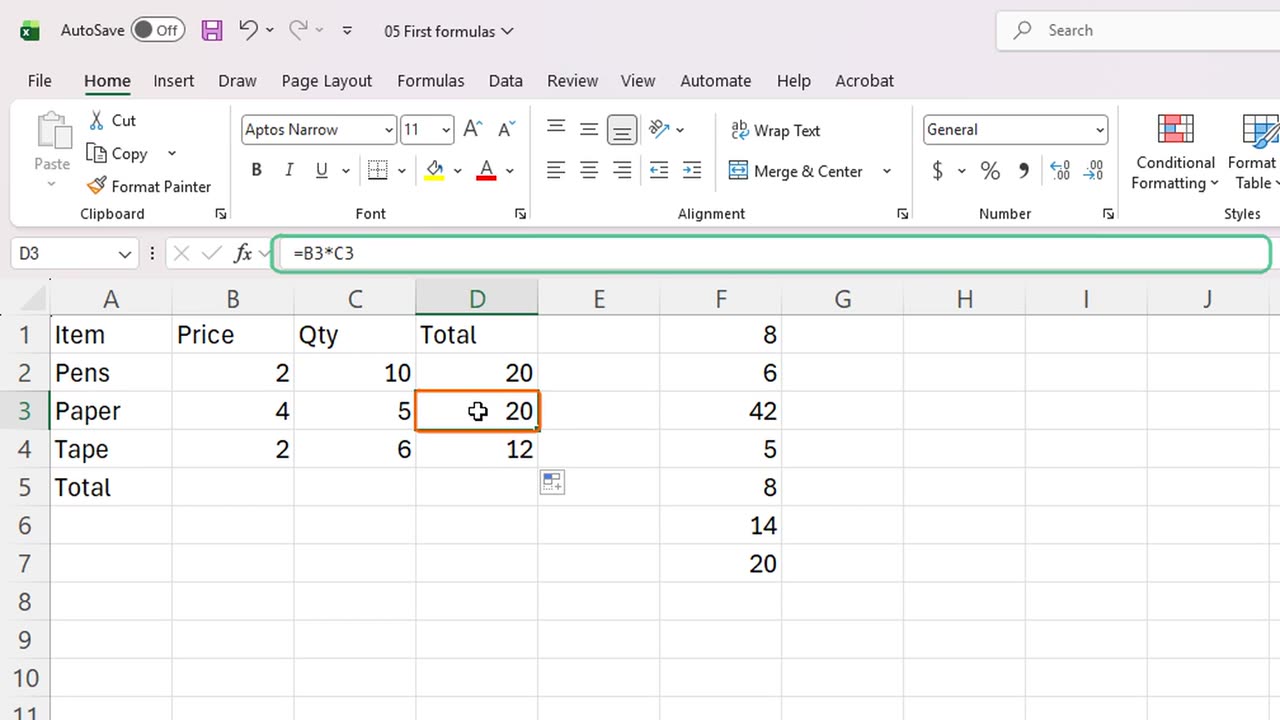
Now we need the same formula for the other rows. Do not retype it. Select D2 and drag the fill handle down to D4.
Excel adjusts the references for every row. Click D3, and you will see equals B3 star C3.
6. A grand total
Let's add a grand total in D5. Type equals D2 plus D3 plus D4, and press Enter.
It works, but adding many cells one by one is slow. In the next lesson, you will meet the SUM function, which does it in one step.
=D2+D3+D4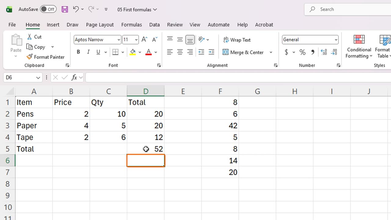
7. Handy formula tools
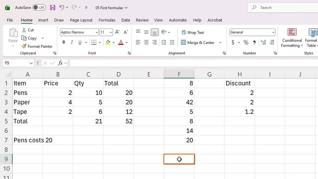
There is a faster way to add: AutoSum. Click C5, under the quantities, and press Alt and the equals sign.
Excel guessed the range, C2 to C4, and wrote a SUM function for us. Press Enter to accept it.
Formulas work with percentages too. In H1 type Discount, and in H2 type equals D2 star zero point one.
Copy it down with the fill handle, and every row gets its own ten percent.
To change a formula, select its cell and press F2. Excel outlines the cells it uses in color. Press Escape to leave without changing anything.
To join text with a formula, use the ampersand. In A7 type equals A2, ampersand, a quoted space costs space, ampersand, D2.
What if something goes wrong? Type equals one slash zero in F9. Dividing by zero is impossible, so Excel shows an error.
Errors are clues, not disasters. We will learn to fix them in the next module. Press Delete to remove this one.
A handy trick: press Control and the backtick key to show every formula in the sheet. Press it again to go back.
=D2*0.1=A2&" costs "&D2=1/0Shortcut: Alt + = Ctrl + `
8. Recap
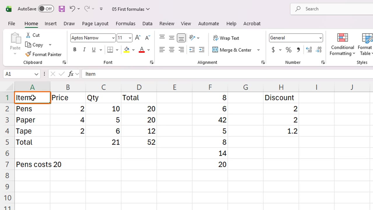
Let's recap. Every formula starts with an equals sign. Use plus, minus, star and slash for the four operations.
Point to cells instead of typing numbers, so the result updates automatically, and drag the fill handle to copy a formula down.
Next time, you will learn the SUM, AVERAGE, MIN, MAX and COUNT functions.
Thanks for watching, and see you in the next lesson.
← Previous tutorial: Select, Copy, Move and AutoFill in Excel (Fast Way)
Next tutorial: Format Text, Numbers and Dates in Excel →