PivotTable Grouping and Calculated Fields
Group dates and numbers, add calculated fields and refresh.
- Months, not dates
- Build the PivotTable
- Group by month
- A calculated field
- The totals trap
- Recap
Step by step
1. Months, not dates
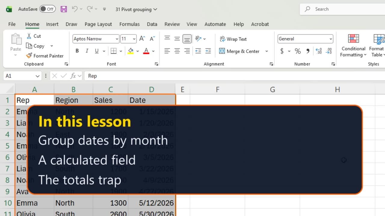
Twelve dates make twelve rows in a PivotTable. Group them, and you get six clean months. Then let the PivotTable calculate a bonus for you.
You will group by month, add a calculated field, and see the one rule that makes calculated fields lie.
2. Build the PivotTable
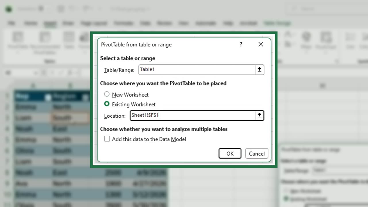
First the PivotTable, built the usual way: Control and T, Enter, then Alt, N, V, T, and place it at F1.
Shortcut: Ctrl + T
3. Group by month
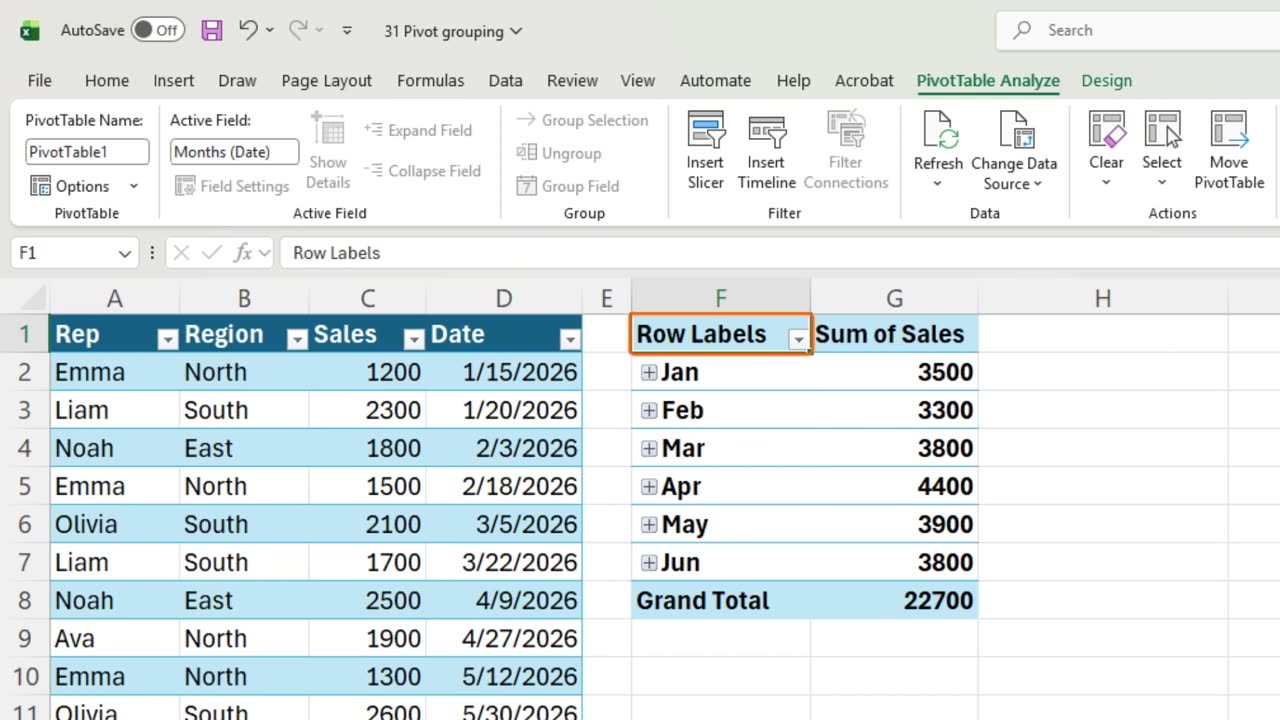
Tick Date. Excel groups the dates into months by itself: Jan to Jun.
Tick Sales. Six months, one total each. January to June, twenty two thousand seven hundred.
If Excel does not group them for you, right-click a date and choose Group, then Months.
4. A calculated field
Now a calculated field: a new column the PivotTable computes from its own fields. Open it with Alt, J, T, J, F.
Name it Commission. In the formula box, type equals Sales times zero point zero five, and click OK.
A new column, five percent of every month. It updates with every refresh, and nothing is added to your data.
Quick pause: if calculated fields are new to you, a like really helps the channel. Because the next part is where they go wrong.
=Sales*0.05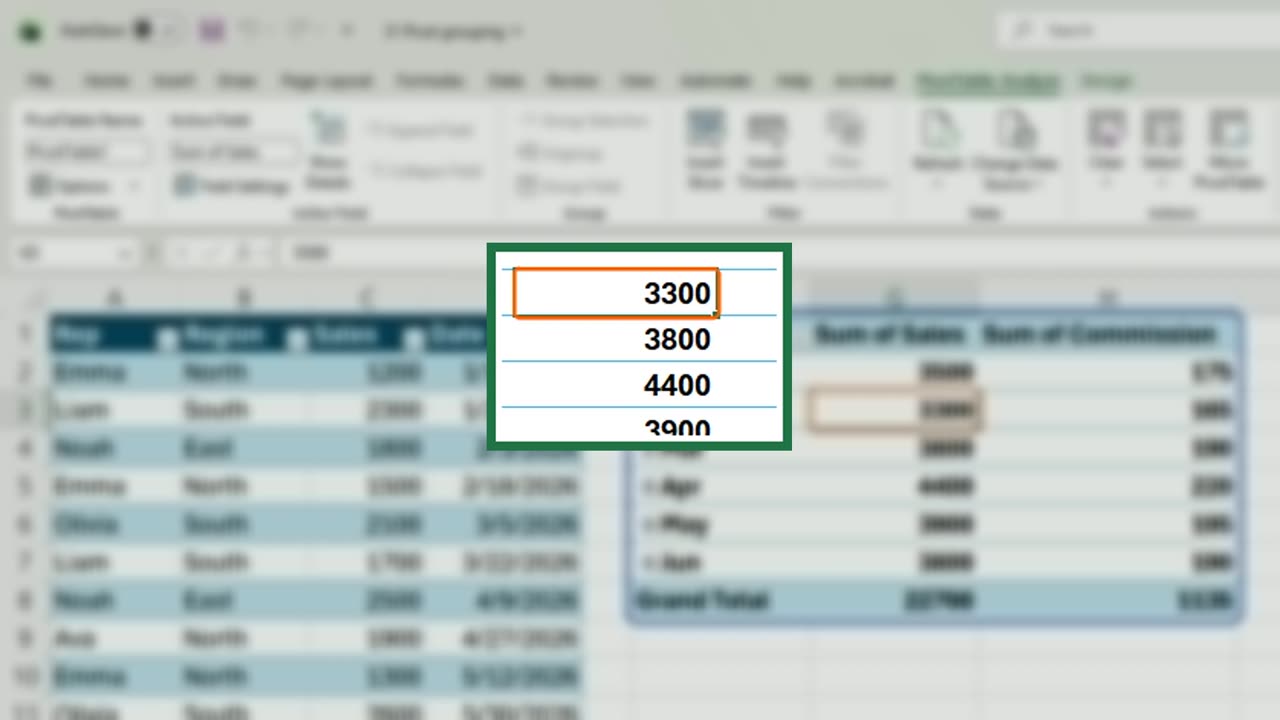
5. The totals trap
Change the rule: only sales over two thousand earn ten percent. Open the dialog again with Alt, J, T, J, F.
Name it Bonus, type equals IF, Sales greater than two thousand, Sales times zero point one, zero, and OK.
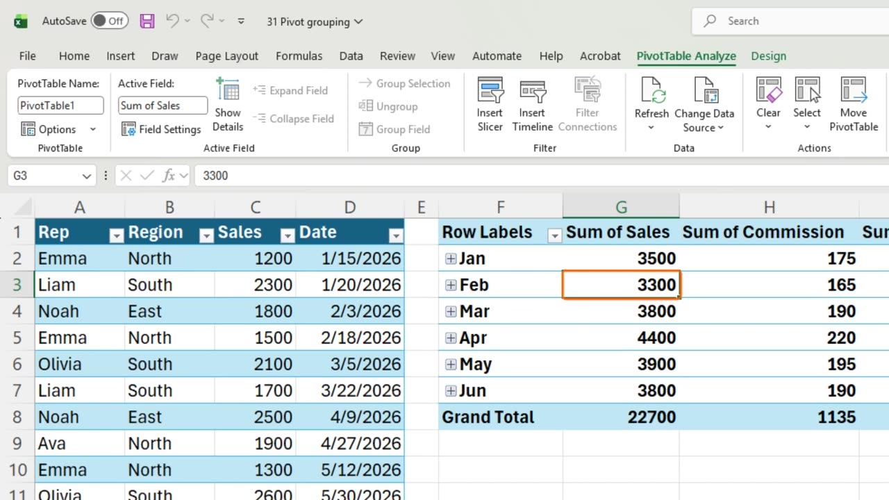
Look at February: a bonus of three hundred thirty. But February's sales were eighteen hundred and fifteen hundred. Neither is over two thousand.
A calculated field never sees single rows. It works on the month's total, three thousand three hundred. For rules per sale, add a column to the Table instead.
=IF(Sales>2000,Sales*0.1,0)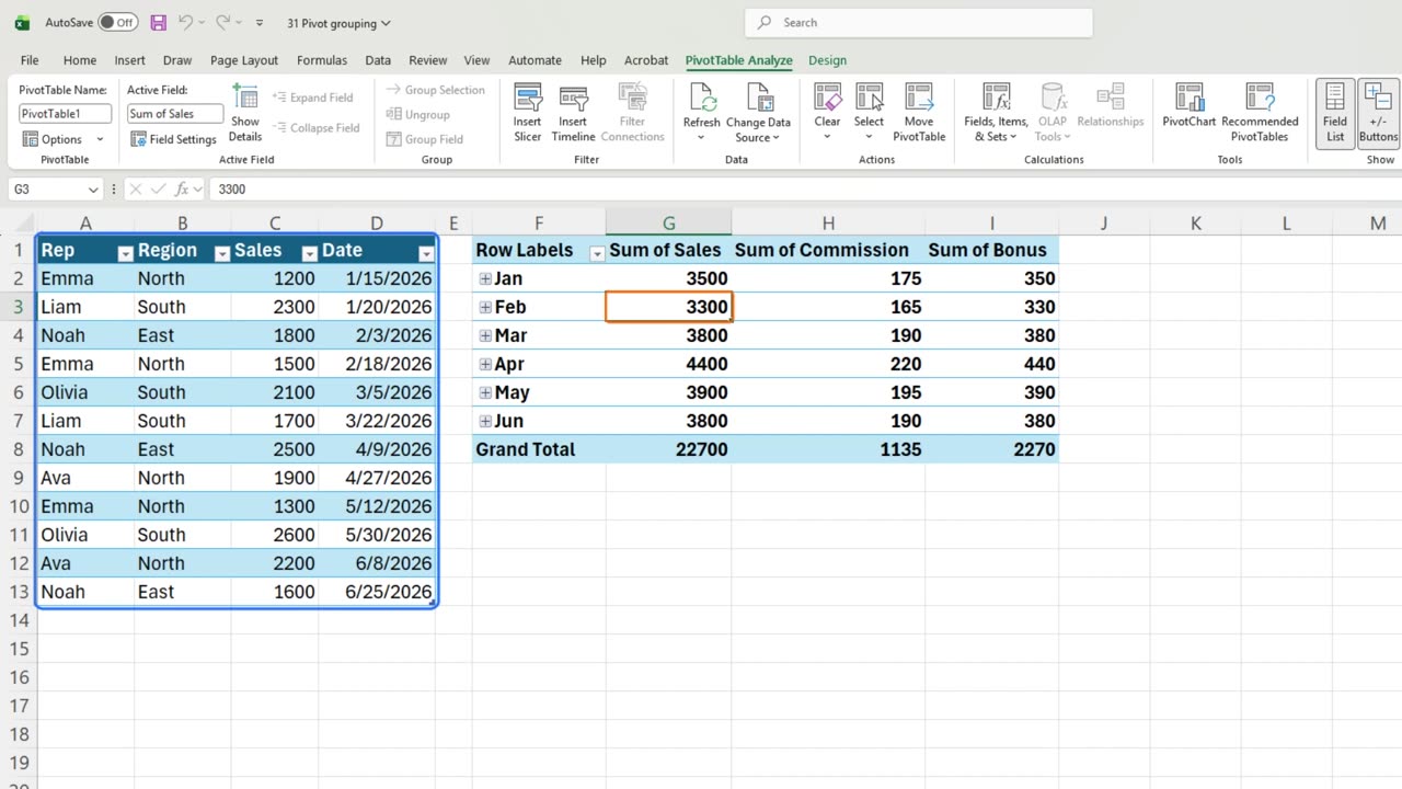
6. Recap
Recap: dates group into months, calculated fields add columns from totals, and rules that test single rows belong in the source Table.
In the next lesson, you will filter a PivotTable with buttons, using slicers.
Have you ever trusted a calculated field that was wrong? Tell me in the comments.
← Previous tutorial: PivotTable Basics in Excel (Step by Step)
Next tutorial: Excel Slicers: Filter PivotTables with Buttons →