PivotTable Basics in Excel (Step by Step)
Summarize thousands of rows with a PivotTable.
- Why PivotTables
- Table first
- Insert a PivotTable
- Rows and values
- The refresh trap
- A second level
- Recap
Step by step
1. Why PivotTables
Twelve sales, three regions. Which region sold the most? With a PivotTable you know in ten seconds, without one formula.
You will build one, add a second level, and learn the refresh trap that fools almost everyone.
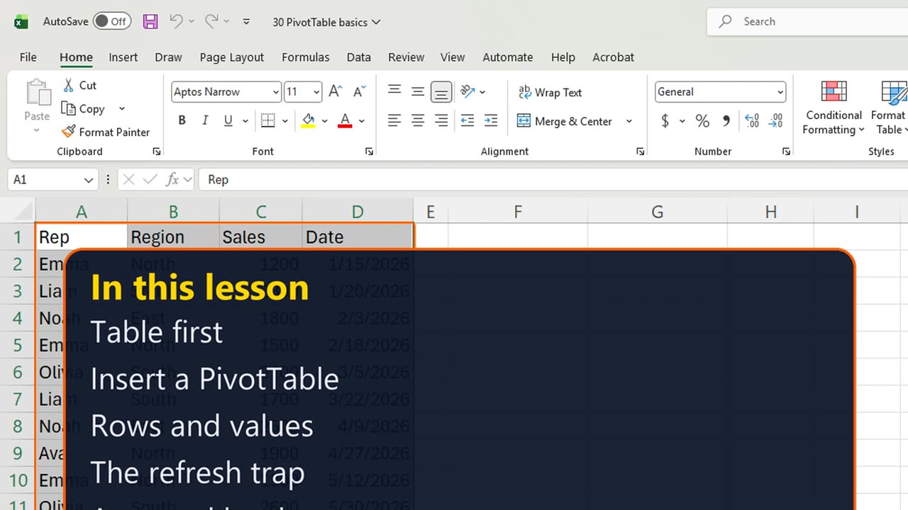
2. Table first
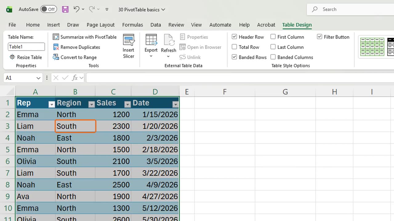
First, turn the data into a Table, so new rows are picked up later. Click inside and press Control and T, then Enter.
Shortcut: Ctrl + T
3. Insert a PivotTable
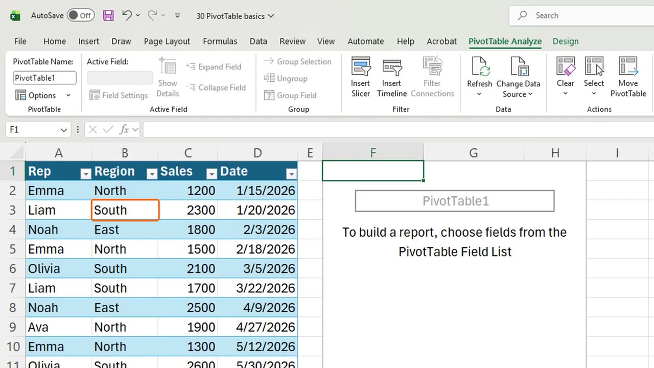
Now Insert, PivotTable: Alt, N, V, T. Excel already picked the Table as the source.
Put it on this sheet: Alt and E for Existing worksheet, Alt and L for the location, type Sheet1, exclamation mark, F1, and Enter.
4. Rows and values
An empty PivotTable, and the field list on the right. Every column of the Table is a field.
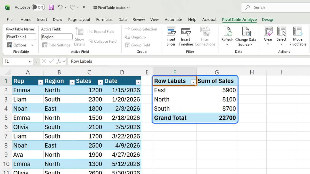
Tick Region. Text fields go to Rows, so each region gets one line.
Tick Sales. Numbers go to Values, and Excel sums them. South sold the most: eight thousand seven hundred.
Quick pause: if you just built your first PivotTable, a like really helps the channel. Now the trap.
5. The refresh trap
A new sale comes in. In A14 type Liam, South, one thousand, and a date, pressing Tab between them.
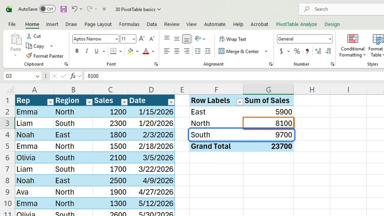
Look at South. Still eight thousand seven hundred. A PivotTable is a snapshot. It does not see new data until you refresh it.
Click inside the PivotTable and press Alt and F5. Now South shows nine thousand seven hundred.
6. A second level
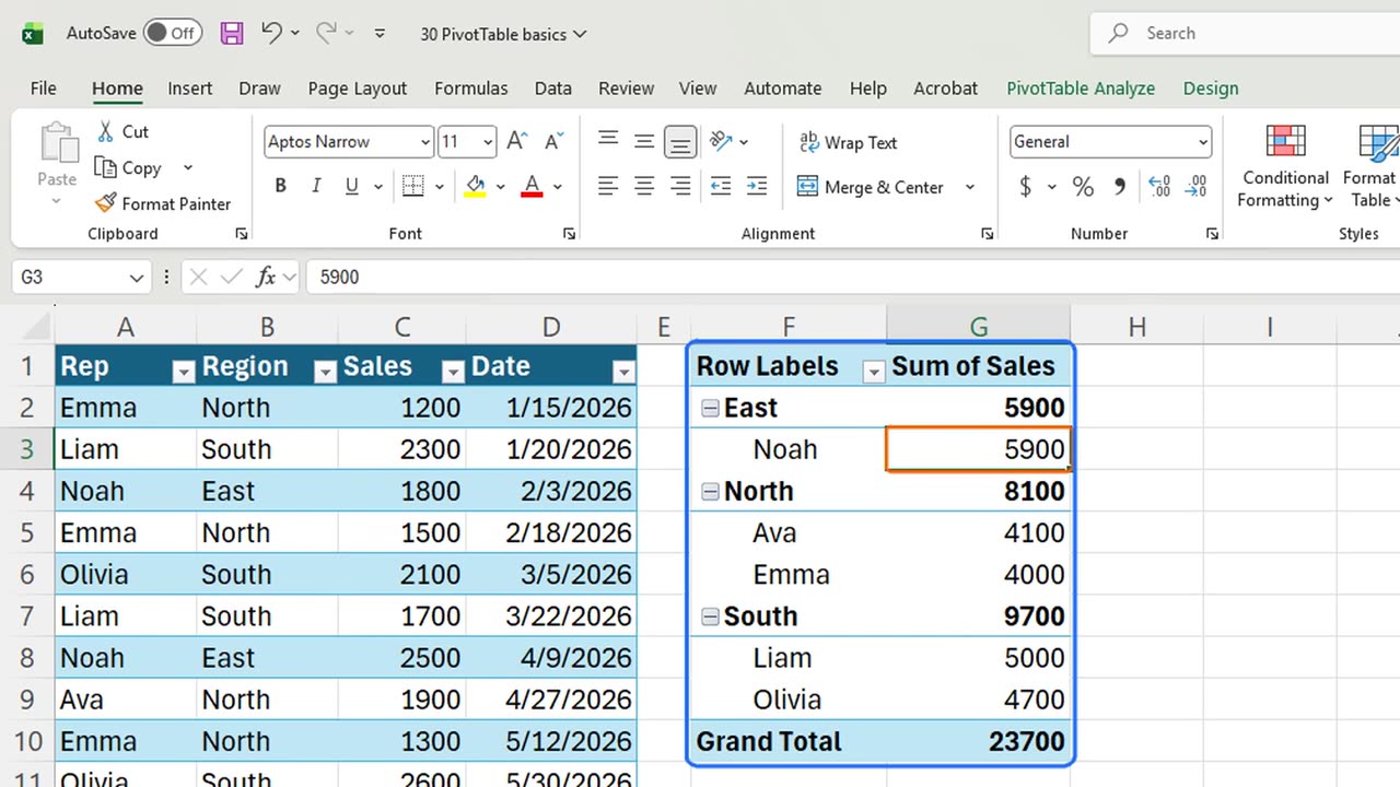
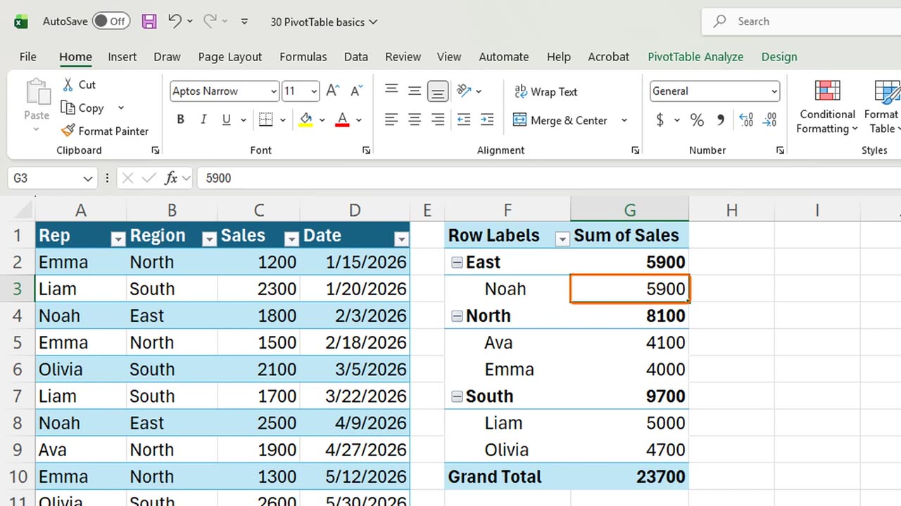
Last, a second level. Tick Rep, and each region opens up into its sales people.
7. Recap
Recap: make a Table, insert a PivotTable, tick a text field for rows and a number for values, and refresh with Alt and F5 after new data.
In the next lesson, you will group dates into months and add a calculated field.
What would you summarize first with a PivotTable at work? Tell me in the comments.
← Previous tutorial: Excel Sparklines: Tiny Charts in a Cell
Next tutorial: PivotTable Grouping and Calculated Fields →