Excel Sparklines: Tiny Charts in a Cell
Show trends inside cells.
- Trends in a cell
- Line sparklines
- High point
- The scale trap
- Column sparklines
- Recap
Step by step
1. Trends in a cell
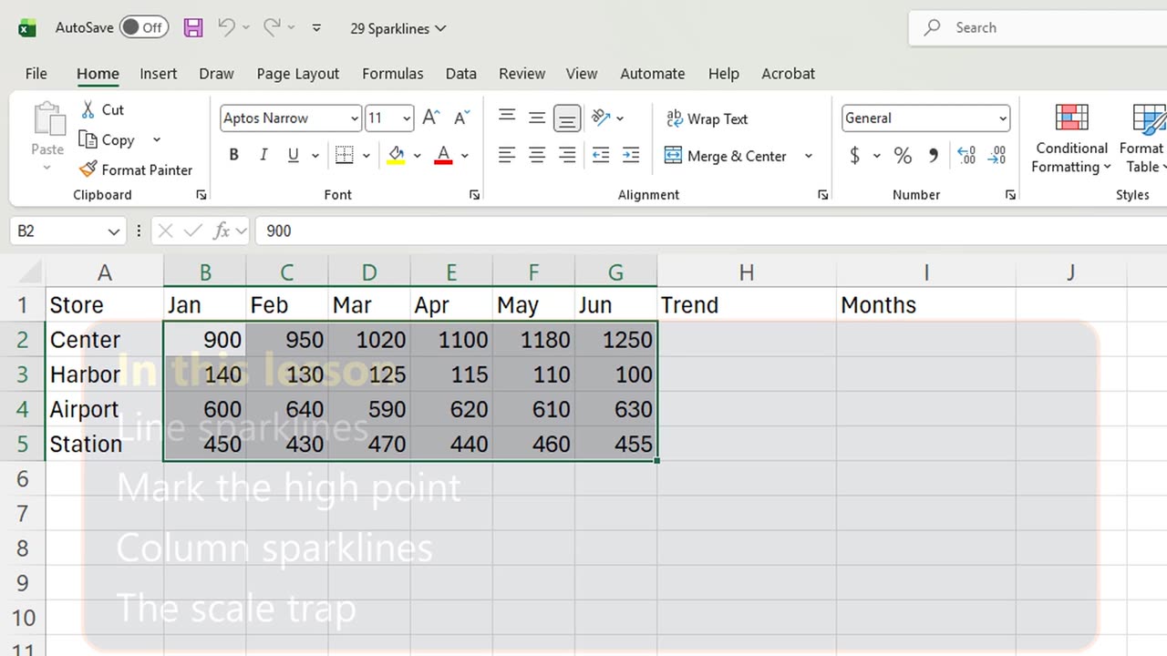
Which store is growing, and which one is slipping? A tiny chart inside each row answers that before you read a single number.
These are sparklines. You will add line sparklines, mark the best month, switch to columns, and fix a scale trap.
2. Line sparklines
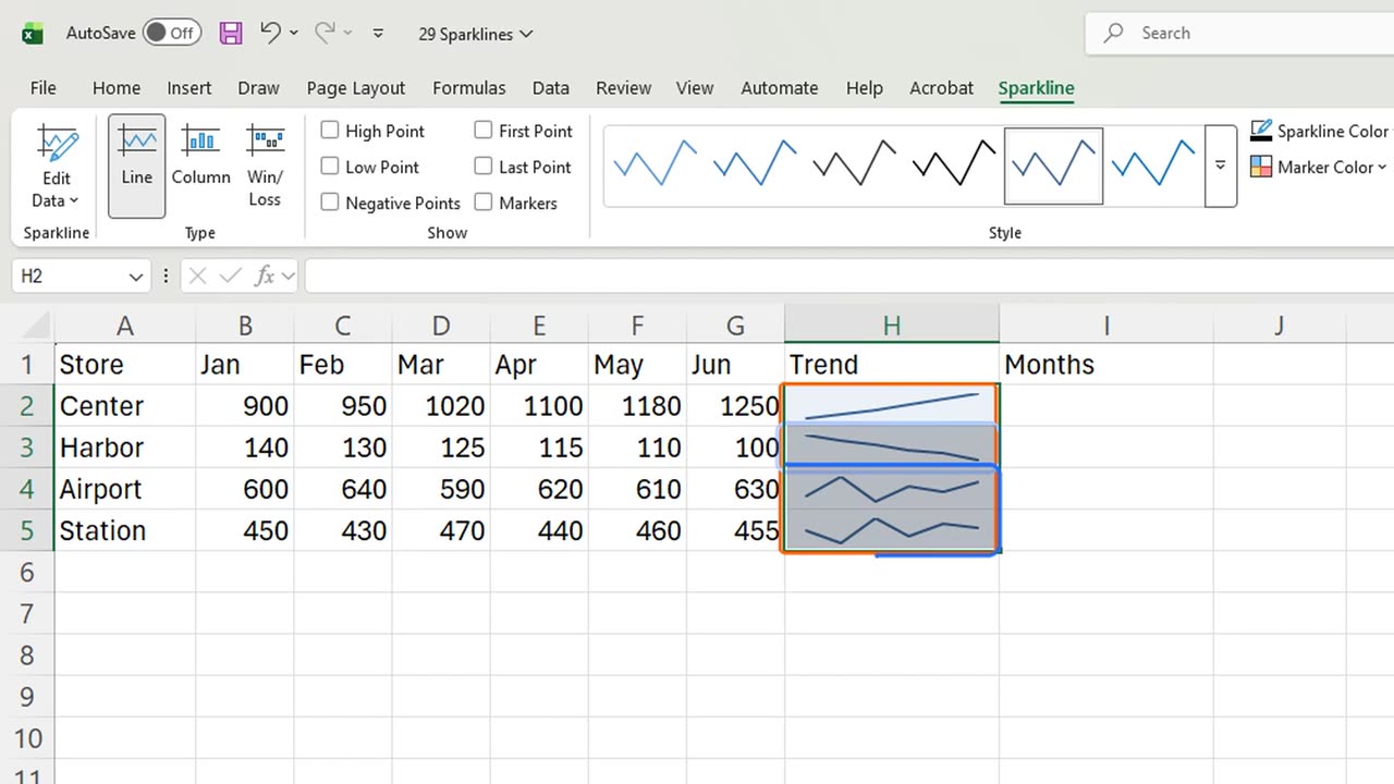
Select H2 to H5, the empty cells where the charts will live. Then Insert, Sparklines, Line: Alt, N, S, L.
Excel knows where they go. It only asks for the data: type B2 colon G5, and press Enter.
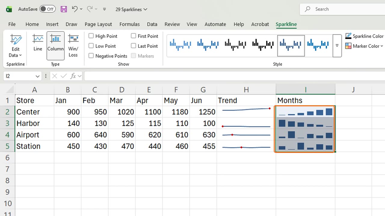
Four rows, four trends. The Center store climbs, the Harbor store falls, and the others move sideways.
3. High point
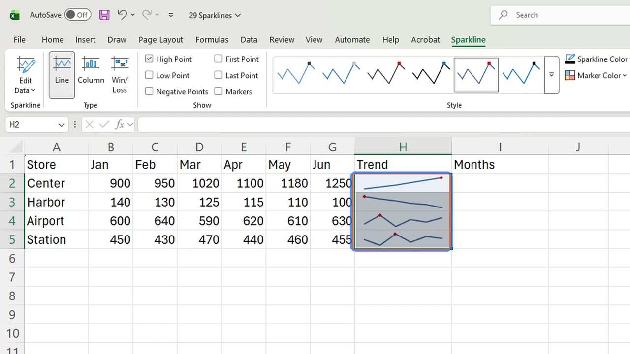
Now mark each store's best month. With the sparklines selected, the Sparkline tab is open. Tick High Point.
Quick pause: if this already saves you a chart, a like really helps the channel. The next part is the trap almost everyone falls into.
4. The scale trap
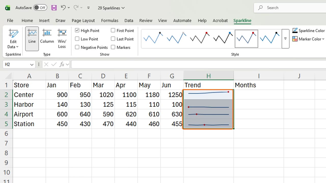
Here it is. Harbor sells about ten times less than Center, yet its line looks just as tall. Each sparkline stretches to its own cell.
Fix it from the Axis button. Choose Same for All Sparklines for the minimum, then open Axis again and do the same for the maximum.
Now Harbor is a flat line near the bottom, the honest size. Compare shapes and sizes together, and you see the real picture.
5. Column sparklines
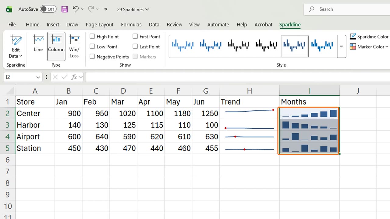
One more type: columns. Select I2 to I5, add line sparklines the same way, then click Column on the Sparkline tab.
Column sparklines compare month by month, line sparklines show the direction. Pick the one that answers your question.
6. Recap
Recap: Alt, N, S, L adds sparklines, High Point marks the best month, Column switches the type, and Same for All Sparklines keeps the sizes honest.
In the next lesson, you will summarize hundreds of rows with your first PivotTable.
Would you rather use sparklines or full charts in your reports? Tell me in the comments.
← Previous tutorial: Format Excel Charts Like a Pro (Titles, Labels, Colors)
Next tutorial: PivotTable Basics in Excel (Step by Step) →