Excel Text Functions: LEFT, RIGHT, MID, LEN, TRIM, CONCAT
Cut, join and clean text with the most useful text functions.
- Intro
- Cutting text
- LEFT
- MID
- RIGHT
- LEN
- TRIM
- CONCAT
- Tips
- Recap
Step by step
1. Intro
Welcome back. In this lesson, you will learn to cut, measure, clean and join text in Excel, using six simple functions: LEFT, MID, RIGHT, LEN, TRIM and CONCAT.
Real data often arrives as messy text: codes that hide several facts, names with extra spaces, and first and last names in separate columns. These functions fix all of that.
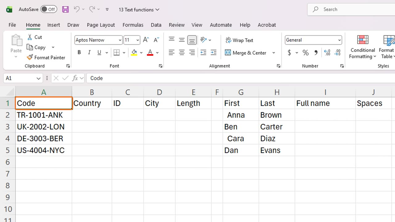
2. Cutting text
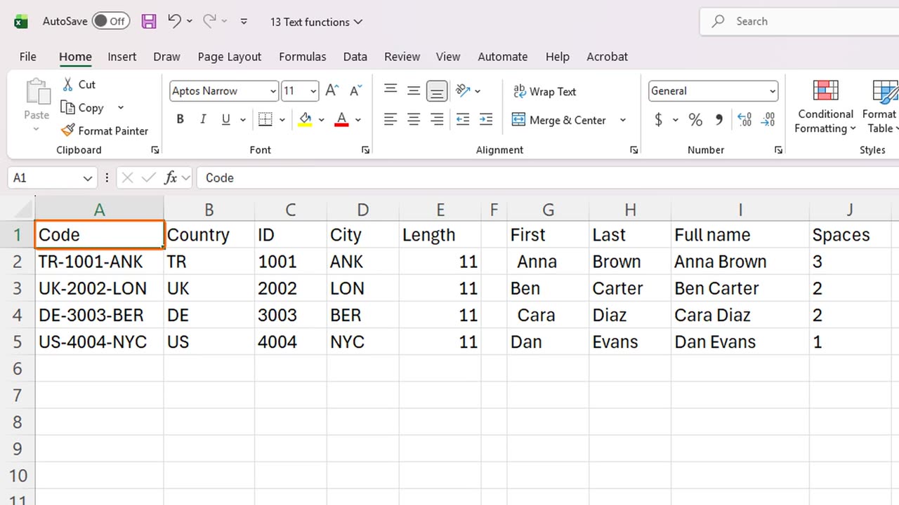
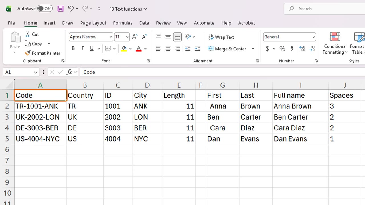
Here are four product codes. Each code hides a country, a number and a city, separated by dashes. Let's pull them apart.
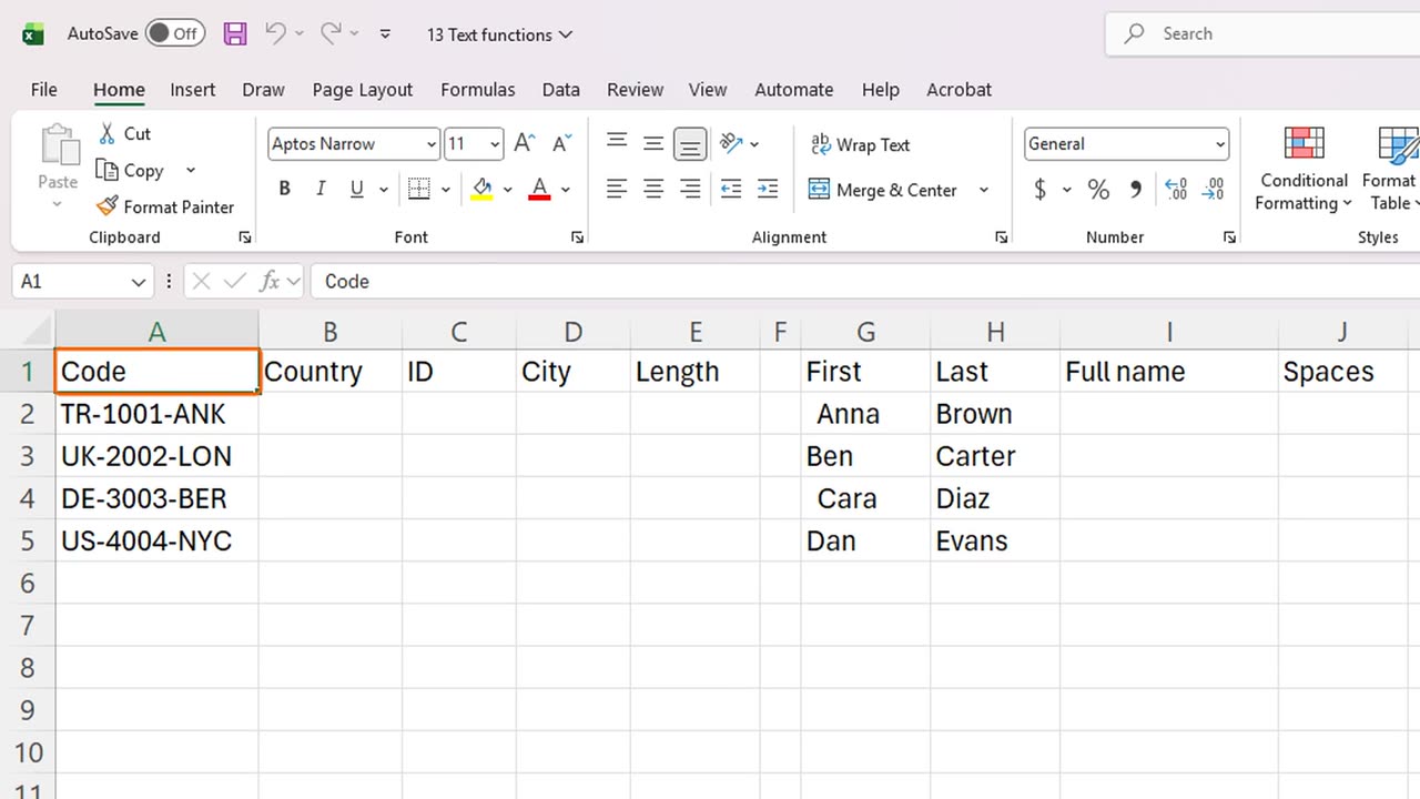
3. LEFT
LEFT takes characters from the start of the text. Click B2 and type equals LEFT, open bracket, A2, comma, 2, close bracket. It means: take the first two characters of A2.
The country code TR appears. Fill the formula down to B5.
=LEFT(A2,2)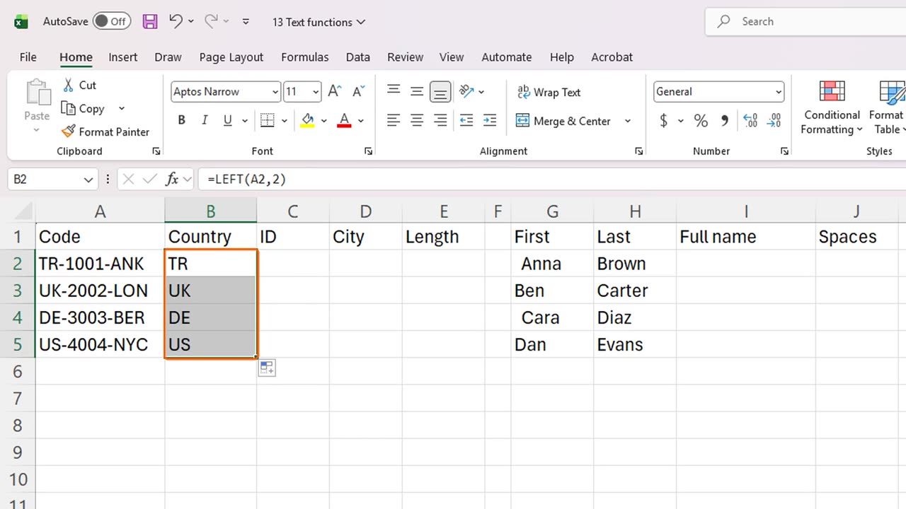
4. MID
MID takes characters from the middle. It needs three things: the text, the starting position, and how many characters. In C2, type equals MID, A2, comma, 4, comma, 4. Start at the fourth character, and take four.
The number one thousand and one appears. Fill it down.
=MID(A2,4,4)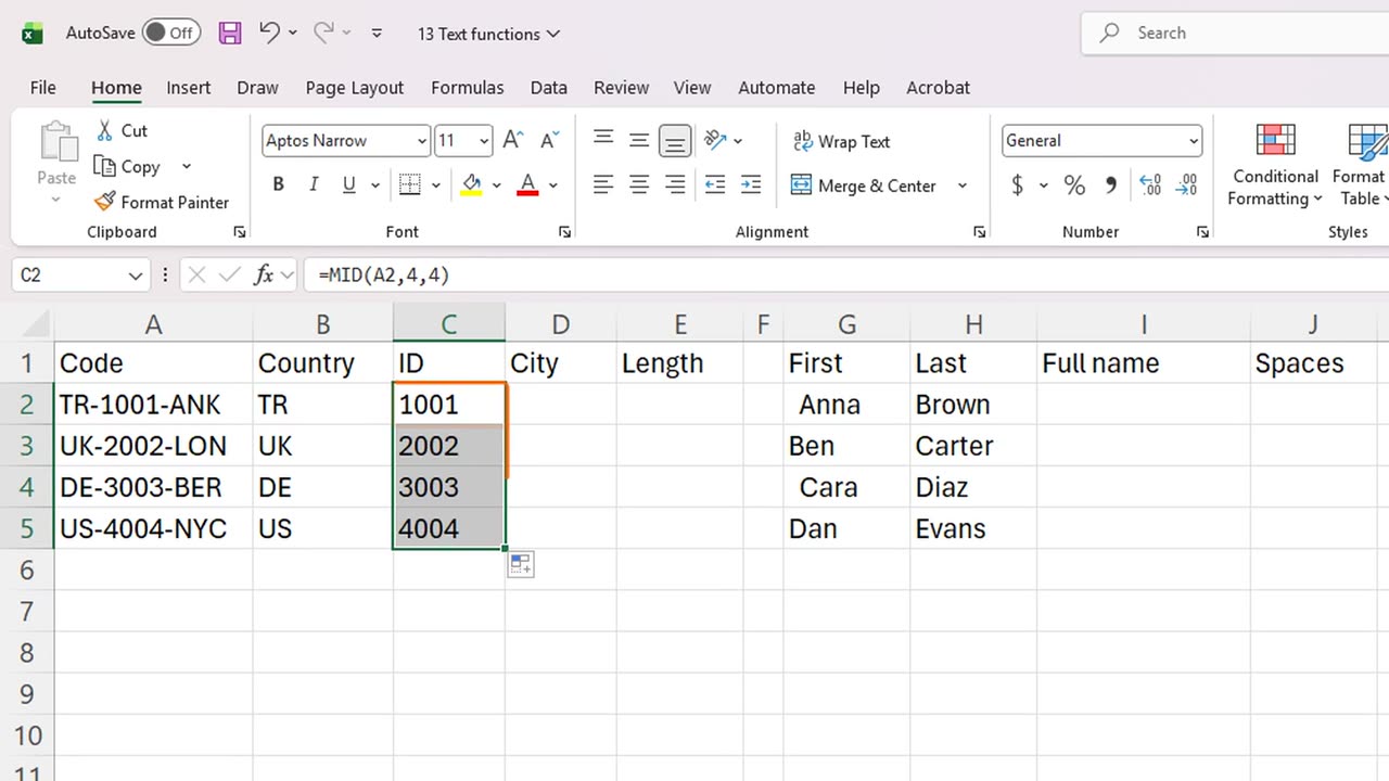
5. RIGHT
RIGHT takes characters from the end. In D2, type equals RIGHT, A2, comma, 3, to get the three letter city code.
Fill it down. LEFT, MID and RIGHT are the three tools for cutting text, and you will use them constantly.
=RIGHT(A2,3)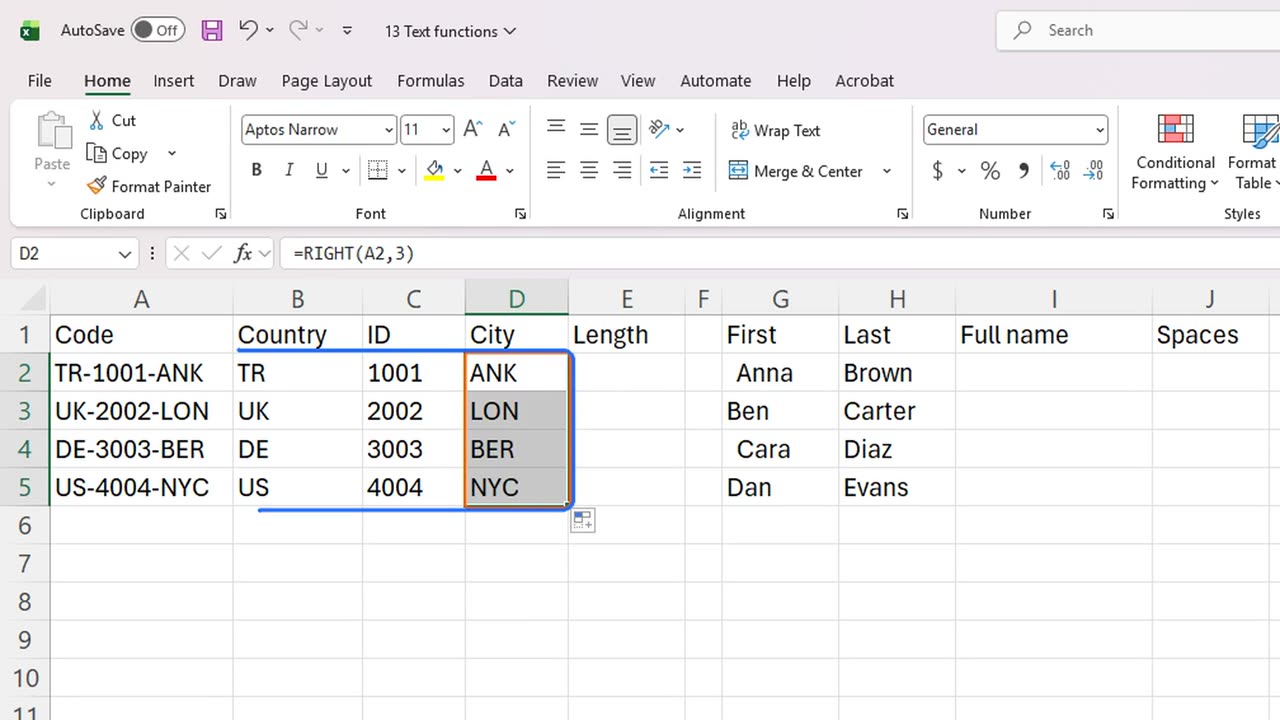
6. LEN
LEN counts the characters in a text, including spaces. In E2, type equals LEN, A2. Every code has eleven characters.
Fill it down. LEN is very useful for checking that codes all have the right length, and, as you will see now, for finding hidden spaces.
=LEN(A2)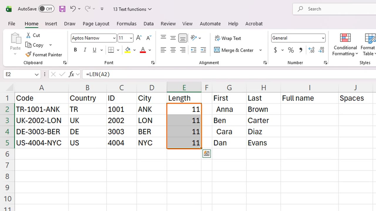
7. TRIM
On the right, there are first names and last names. Some first names have extra spaces that you cannot see.
Let's find them. In J2, type equals LEN of G2 minus LEN of TRIM of G2. TRIM removes extra spaces, so the difference is the number of spaces removed.
Anna has three extra spaces. Fill it down, and you see which names are dirty.
TRIM removes spaces at the start and at the end, and reduces double spaces in the middle to one. It is the first thing to try when a lookup fails for no obvious reason.
=LEN(G2)-LEN(TRIM(G2))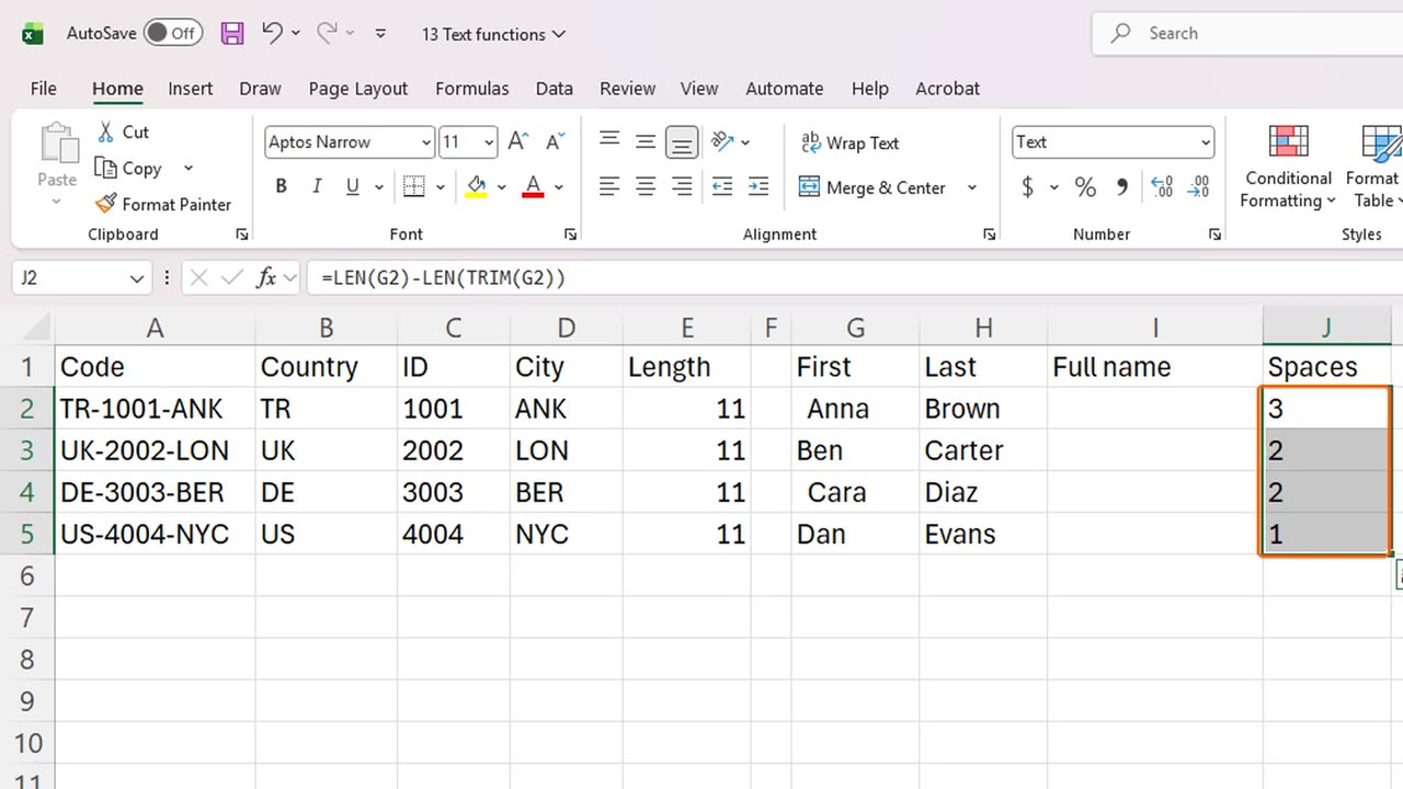
8. CONCAT
Now let's join the names. CONCAT glues text together. In I2, type equals CONCAT, open bracket, TRIM of G2, comma, a space in quotes, comma, H2, close bracket.
We trimmed the first name, added a space between the two parts, and joined the last name. Fill it down, and the full names are clean and tidy.
Notice how we combined two functions, CONCAT with TRIM inside it. You can nest functions like this, and Excel works from the inside out.
There is a shorter way to join text: the ampersand symbol. Equals A1 and quote, dash, quote, and B1 gives the same result as CONCAT. Use whichever you find easier to read.
=CONCAT(TRIM(G2)," ",H2)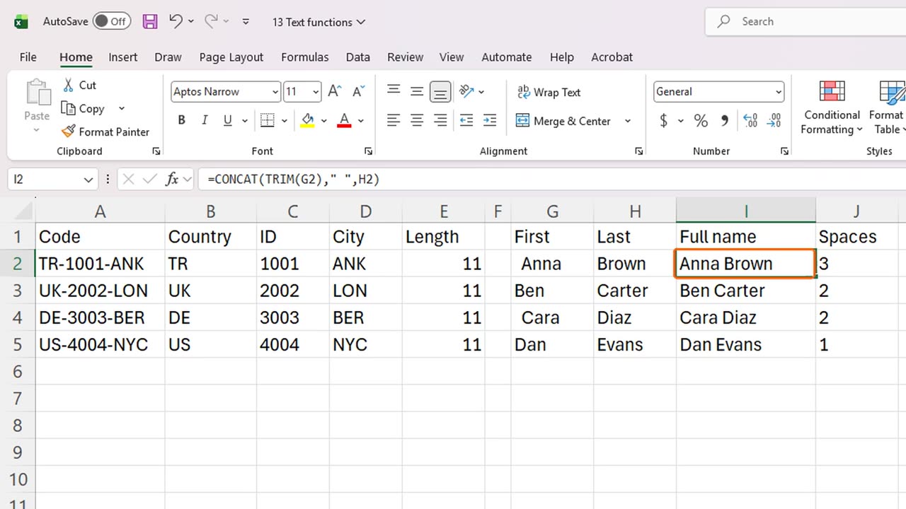
9. Tips
Here are three tips. Text functions always return text, so a number cut with MID is stored as text. Positions start counting at one, not zero. And always test your formula on the first row before you fill it down.
10. Recap
Let's recap. LEFT, MID and RIGHT cut text. LEN counts characters. TRIM removes extra spaces. And CONCAT joins pieces together.
Next time, you will work with dates: TODAY, NOW, DATEDIF and EOMONTH.
If there is something you want to learn next, write it in the comments. Your requests decide what we teach in the next tutorials. Thanks for watching, and see you in the next one.
← Previous tutorial: Excel IF Function for Beginners (with Examples)
Next tutorial: Excel Date Functions: TODAY, NOW, DATEDIF, EOMONTH →